
Localizing Predetermined Objects Underwater Using Stereo Vision
Published:
View this project on Github: ROS Wrapper for entire image pipeline ROS Wrapper for StereoAdapter
Introduction
Localizing a known object in three-dimensional space is a prerequisite for any manipulation or navigation task that requires a robot to act on its environment. Underwater, this problem is considerably harder than in air: the medium introduces light scattering, colour attenuation, and a near-uniform visual texture that confounds most standard depth-estimation pipelines.
This write-up documents a three-stage investigation into stereo-based localization for predetermined underwater objects. The approach begins with the standard ROS stereo_image_proc pipeline using Semi-Global Block Matching (SGBM), moves through a deep-learning depth predictor (StereoAdapter) motivated by the Controls team’s 3D mapping work, and returns to a refined classical pipeline combining noise filtering, image enhancement, and empirical polynomial reprojection. Each stage is honest about where it broke down and why, because those failures directly motivated what came next.
Stage 1: Baseline Disparity with SGBM
1.1 Setup
The starting point was stereo_image_proc, the standard ROS package for rectifying stereo pairs and computing disparity maps. Within this package, two algorithms were available:
- SGBM (Semi-Global Block Matching)
- SGM (Semi-Global Matching)
SGBM was selected first because initial tests showed it produced a denser disparity map — more pixels were assigned valid depth estimates compared to SGM, which left larger regions undefined. A denser map was assumed to be more useful downstream for localization.
1.2 The Underwater Noise Problem
The disparity map produced by SGBM was immediately affected by the underwater environment. Block matching algorithms work by finding regions of one image inside the other; they depend on local texture being distinctive enough to identify correspondences. Underwater scenes are the opposite of this: suspended particles, caustic lighting, and the near-featureless appearance of sand, water column, and structural surfaces all produce texture ambiguity — many regions look indistinguishable from one another within the matching window.
The result was a disparity map saturated with spurious readings. Valid depth estimates were present, but they were buried inside a dense field of noise that made direct use of the raw output unreliable.
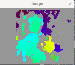
Figure 1. SGBM disparity map computed on the author. The general shape of the face is discernible, confirming that the algorithm can recover structure when sufficient local contrast is present — but the surrounding regions are filled with noisy, unreliable readings.
A note on this stage. No systematic evaluation of SGBM noise levels was carried out at this point, and no quantitative metrics were recorded. The decision to move on was based on qualitative inspection of the disparity output on underwater footage, where the signal-to-noise ratio was assessed as too low to proceed without intervention.
Stage 2: Deep Learning Depth Estimation with StereoAdapter
2.1 Motivation
The Controls team had been pursuing environment-aware navigation using a 3D point cloud model of the vehicle’s surroundings. This created a natural motivation to try a learning-based stereo depth estimator: if a model trained on diverse scene types could generalise to the underwater domain, it might sidestep the texture-ambiguity problem that broke SGBM — deep features are less dependent on local texture contrast than handcrafted matching windows.
StereoAdapter was selected as the candidate model. It adapts pretrained monocular depth features for use with stereo pairs, allowing it to leverage rich learned priors while still exploiting the geometric constraints of a calibrated stereo rig.
2.2 Qualitative Results
The model was run on captured underwater frames. Depth maps and derived 3D point clouds were generated and inspected qualitatively.
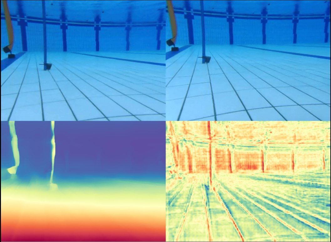
Figure 2. StereoAdapter depth estimate on an underwater scene. The model recovers plausible scene geometry where SGBM produced noise.
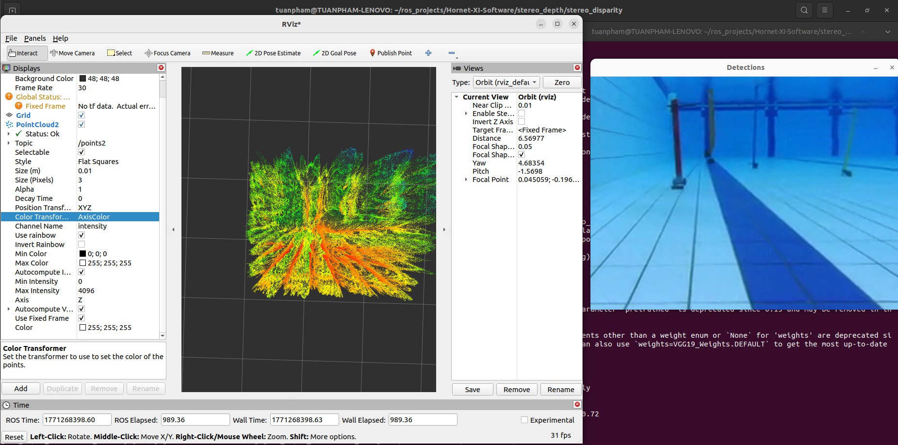
Figure 3. 3D point cloud reconstructed from StereoAdapter depth estimates. Structure in the scene is visible, though fidelity near featureless surfaces is limited.
2.3 The Compute Bottleneck
The fundamental obstacle was inference latency. Processing a single stereo frame through StereoAdapter took approximately 1 second on the available hardware. For any real-time localization loop — which must track a moving object and feed control signals continuously — this throughput is not viable. The minimum acceptable frame rate for the downstream task is well above 1 Hz.
This stage concluded that StereoAdapter is a useful diagnostic tool for understanding scene structure offline, but it cannot be deployed on hardware in its current form without access to significantly more compute. Optimisation paths such as model quantisation or ONNX export were considered but not pursued, as the classical pipeline had not yet been exhausted.
Stage 3: Refined Classical Pipeline
Given the failure modes of the previous two stages — raw SGBM noise and StereoAdapter latency — Stage 3 returned to stereo_image_proc with two targeted interventions: a noise-reduction strategy applied to the disparity output, and an empirical reprojection model to correct for the systematic biases introduced by the underwater medium.
3.1 Disparity Noise Reduction
Algorithm Change: SGBM → SGM
The first change was switching the disparity algorithm from SGBM to SGM. While SGBM returned more raw disparity points, many of those additional points were noise. SGM is more conservative: it assigns fewer valid estimates, but the ones it does assign are more reliable. When the downstream step filters points to only those inside known bounding boxes (the predetermined object regions), the absolute count of valid points matters less than their quality.
Bounding-Box Masking
After disparity computation, only the points falling inside the bounding box of the target object are retained. Points outside the box are discarded entirely. This is a straightforward step, but it is necessary to prevent the large volume of background noise from overwhelming any subsequent statistical filtering.
Median Absolute Deviation Filtering
Even within the bounding box, outliers remain. Median Absolute Deviation (MAD) filtering was applied to the retained disparity values:
\[\text{MAD} = \text{median}(|x_i - \tilde{x}|)\]Points further than a threshold multiple of the MAD from the median are rejected. MAD is preferred over standard deviation here because it is robust to the heavy-tailed distributions that noisy disparity data tends to produce — standard deviation is inflated by large outliers, causing it to mask them rather than reject them.
Image Preprocessing: CLAHE and Histogram Stretching
One root cause of sparse and noisy disparity in low-contrast underwater scenes is that the input images lack the local intensity variation needed for block matching to find reliable correspondences. Two preprocessing steps were added to address this before disparity computation:
- CLAHE (Contrast Limited Adaptive Histogram Equalisation): Enhances local contrast across the image by equalising intensity distributions within small tiles, rather than globally. The contrast limit prevents over-amplification of noise in uniform regions.
- Histogram Stretching: Linearly rescales the intensity range to span the full available dynamic range, recovering contrast lost to the absorptive and scattering properties of water.
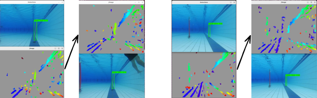
Figure 4. Comparison of valid disparity points inside the bounding box before and after applying CLAHE and histogram stretching. Preprocessing increases the number of usable points the algorithm can recover from the scene.
The improvement shown in Figure 4 confirms that the sparsity problem in Stage 1 was partly a consequence of poor input contrast, not solely an algorithmic limitation of SGBM. Providing better-conditioned images to the matcher meaningfully increases the density of valid, in-box points.
3.2 Empirical Reprojection Fitting
Motivation
Even a clean disparity reading does not directly yield a metric depth in water. Standard stereo reprojection assumes the propagation geometry of air. Underwater, refraction at the camera housing interface and the altered index of refraction introduce systematic errors that grow with distance. These errors are not easily corrected with a closed-form model unless the exact housing geometry and port type are known precisely.
An empirical approach was taken instead: collect ground truth distance measurements at a range of known distances, record the corresponding raw disparity or reprojected depth readings, and fit a corrective function.
Ground Truth Collection
A calibration target was placed at multiple known distances from the stereo rig. At each position, depth readings from the pipeline were recorded and compared against the physically measured ground truth.
Polynomial Fitting
Two corrective models were fitted to the collected data:
- First-order (linear) fit: $\hat{d} = a_1 x + a_0$
- Second-order (quadratic) fit: $\hat{d} = a_2 x^2 + a_1 x + a_0$
where $x$ is the raw pipeline output and $\hat{d}$ is the corrected depth estimate.
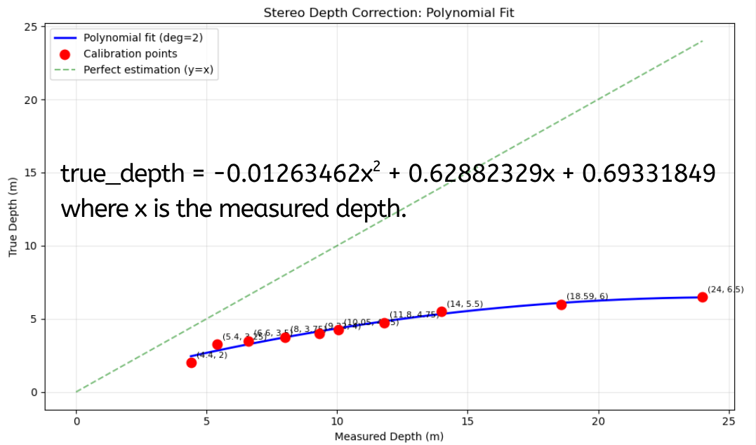
Figure 5. First-order polynomial fit between raw pipeline depth readings and ground truth distances. A linear relationship is a reasonable approximation across the measured range.
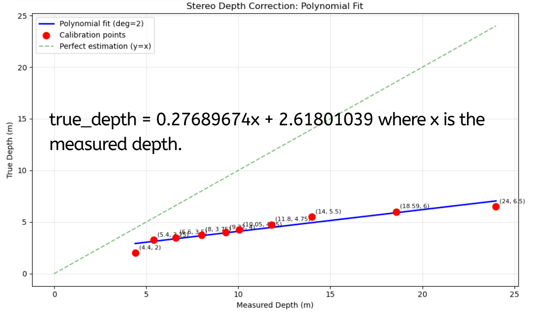
Figure 6. Second-order polynomial fit. The additional degree of freedom allows the model to account for the nonlinear error growth at longer ranges that a linear model cannot capture.
The second-order fit captures the nonlinear component of the underwater reprojection error — at longer distances, the systematic bias increases faster than a linear function of distance, which aligns with the physics of refraction errors growing with the angle subtended by the light path through the housing.
Limitations of the calibration data. The ground truth measurements were collected at a limited number of discrete distances. The fitted polynomials interpolate between these points but do not account for variation with lateral position in the frame, temperature-dependent changes in the refractive index of water, or turbidity. The calibration should be treated as a first-order correction rather than a precise underwater reprojection model.
Summary
The three stages represent a progression from a naive baseline through a compute-limited deep learning detour and back to a refined classical pipeline:
| Stage | Method | Core Problem | Outcome |
|---|---|---|---|
| 1 | SGBM via stereo_image_proc | Noise dominates in low-texture underwater scenes | Too noisy to use directly |
| 2 | StereoAdapter deep estimator | ~1 s per frame on available hardware | Not viable for real-time deployment |
| 3a | SGM + MAD filtering + CLAHE/Histogram Stretching | Noisy in-box readings, sparse correspondences | Improved point quality and density |
| 3b | Empirical polynomial reprojection | Systematic underwater depth bias | First- and second-order correction applied |
The refined pipeline in Stage 3 is not a final solution — the calibration data is sparse, and the preprocessing pipeline has been validated qualitatively more than quantitatively. But it is a working system that runs within the compute budget and produces depth estimates that are at least corrected for the dominant sources of underwater error.
Limitations and Future Work
Calibration Coverage
The empirical reprojection fitting was performed at a small number of ground truth distances. A more robust calibration would sample densely across the operational range, include off-axis positions to characterise field-position-dependent distortion, and be repeated under different water conditions (turbidity, temperature) to assess sensitivity.
Bounding Box Dependency
The entire noise-reduction strategy depends on having reliable bounding boxes around the target objects before depth estimation. If the object detector fails or produces imprecise boxes, the masking step may include noisy background points or exclude valid object points. The localization pipeline is therefore only as robust as the upstream detection.
Generalisation to Moving Targets
All calibration and testing was performed on stationary targets. Localizing objects in motion introduces temporal consistency requirements — a single noisy frame can cause a large apparent position jump. Temporal filtering (e.g., a Kalman filter over the depth estimates) was not implemented and represents an important next step.
StereoAdapter on Dedicated Hardware
The compute bottleneck in Stage 2 was a hardware constraint, not a fundamental limit of the approach. Running StereoAdapter on a GPU-equipped embedded board, or exporting the model to a quantised inference format (e.g., TensorRT), could make real-time deep learning depth estimation viable. If the accuracy advantage over the classical pipeline is confirmed quantitatively, this path is worth revisiting.
Conclusion
This project worked through the practical difficulty of stereo-based depth estimation in an underwater environment where the standard assumptions of stereo vision — rich texture, air as the propagation medium, consistent illumination — do not hold.
The central finding is that neither a raw classical pipeline nor a pretrained deep estimator is sufficient on its own. SGBM provides a fast, deployable baseline but is overwhelmed by underwater noise. StereoAdapter offers better robustness to texture ambiguity but cannot currently meet real-time constraints on the available hardware. The refined Stage 3 pipeline is a pragmatic combination: conservative disparity estimation, statistical outlier rejection, contrast enhancement on the input, and an empirically fitted correction for the systematic underwater depth bias.
The methodological lesson that carries forward is that the underwater domain violates enough assumptions of standard stereo pipelines that domain-specific validation at every step is not optional. Each component — the disparity algorithm, the preprocessing, the reprojection model — required underwater-specific tuning or replacement. A pipeline assembled from components validated only in air will not transfer reliably.