
Image Inpainting with Deep Learning: Convolutional Autoencoders and Vision Transformers
Published:
Introduction
Image inpainting is the task of reconstructing missing or corrupted regions of an image so that the result is visually coherent with its surroundings. This project explores two deep learning architectures for this task: a Convolutional Autoencoder (CAE) and a Vision Transformer (ViT). Both models are trained to accept an image with artificially blacked-out regions and output a complete reconstruction.
The project is divided into two parts. Part A systematically evaluates design choices for the CAE — optimizer selection, latent dimensionality, and masking strategy — using the CIFAR-10 dataset. Part B takes the lessons learned from Part A and applies them to a more expressive ViT architecture, trained on the Oxford-IIIT Pet Dataset. Wherever single-run constraints limited statistical certainty, this is explicitly stated rather than overstated.
Part A: Convolutional Autoencoder
1. Overview
A Convolutional Autoencoder compresses an input image into a compact latent representation (encoding) and then reconstructs the full image from that representation (decoding). When the input is a corrupted version of the original, the model is forced to use the surrounding context to infer the missing region — the core mechanism behind learning-based inpainting.
1.1 Dataset
All CAE experiments use the CIFAR-10 dataset, which contains 60,000 colour images of size 32×32 across 10 classes: airplanes, cars, birds, cats, deer, dogs, frogs, horses, ships, and trucks.
The dataset is partitioned as follows:
| Split | Images | Purpose |
|---|---|---|
| Training | 45,000 | Gradient updates |
| Validation | 5,000 | Monitoring generalisation |
| Test | 10,000 | Final held-out evaluation |
This split provides a sufficiently large validation set to detect overfitting without reducing training data excessively.
1.2 Data Preprocessing: Simulating Occlusions
To create training pairs, a binary mask is applied to each image before it is passed to the model. The ground-truth unmasked image serves as the reconstruction target.
In the baseline configuration, a single 10×10 black square (100 pixels, ~9.8% of the 32×32 image) is placed at a random location within the image boundary. This forces the model to infer the masked region from its surroundings without any shortcut.
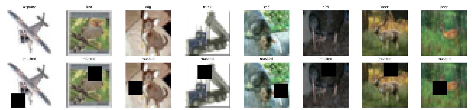
Figure 1. Examples of CIFAR-10 images with a randomly placed 10×10 occlusion mask.
1.3 Model Architecture
The CAE consists of a three-layer encoder and a symmetric three-layer decoder.
Encoder. Three stride-2 convolutional layers progressively halve the spatial resolution while expanding the channel depth: spatial dimensions shrink from 32→16→8→4, and channels grow from 3→32→64→latent_channels. The result is a compact latent tensor of shape (latent_channels, 4, 4).
Decoder. Three transposed convolutional layers mirror the encoder in reverse, upsampling from 4→8→16→32 while reducing channels from latent_channels→64→32→3. A Tanh activation on the final layer constrains output values to [−1, 1], matching the normalised input range.
self.encoder = nn.Sequential(
    nn.Conv2d(3, 32, kernel_size=3, stride=2, padding=1),   nn.ReLU(),
    nn.Conv2d(32, 64, kernel_size=3, stride=2, padding=1),  nn.ReLU(),
    nn.Conv2d(64, latent_channels, kernel_size=3, stride=2, padding=1), nn.ReLU()
)

self.decoder = nn.Sequential(
    nn.ConvTranspose2d(latent_channels, 64, kernel_size=3, stride=2, padding=1, output_padding=1), nn.ReLU(),
    nn.ConvTranspose2d(64, 32, kernel_size=3, stride=2, padding=1, output_padding=1),             nn.ReLU(),
    nn.ConvTranspose2d(32, 3,  kernel_size=3, stride=2, padding=1, output_padding=1),             nn.Tanh()
)
Stride-2 convolutions were chosen over pooling layers because they are learnable and preserve more spatial information during downsampling, which is especially important for a reconstruction task. ReLU activations introduce non-linearity while remaining computationally efficient and avoiding the vanishing gradient problems of sigmoid or tanh in intermediate layers.
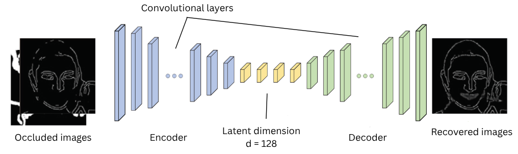
Figure 2. Baseline CAE architecture: encoder (left) compresses to latent space; decoder (right) reconstructs.
Loss function. The network minimises Mean Squared Error (MSE) between its output and the original clean image. MSE was chosen as the baseline loss because it is differentiable everywhere and directly penalises pixel-level reconstruction error. Its limitations (tendency to produce blurred outputs) are discussed in Section 3.
Baseline hyperparameters:
| Hyperparameter | Value |
|---|---|
| Loss Function | MSE |
| Activation | ReLU |
| Optimizer | Adam |
| Latent Channels | 128 |
| Epochs | 200 |
| Batch Size | 256 |
| Learning Rate | 0.001 |
| Mask Size | 10×10 pixels |
| Trainable Parameters | 186,371 |
2. Results and Discussion
A note on experimental scope. Each configuration was trained once due to project timeline constraints. Reported MSE values are therefore point estimates without confidence intervals. Where differences between configurations are small (< 0.001), they should be interpreted cautiously. Larger differences (e.g., SGD vs. Adam) are unlikely to reverse under repeated runs and are discussed with greater confidence.
2.1 Baseline Model Performance
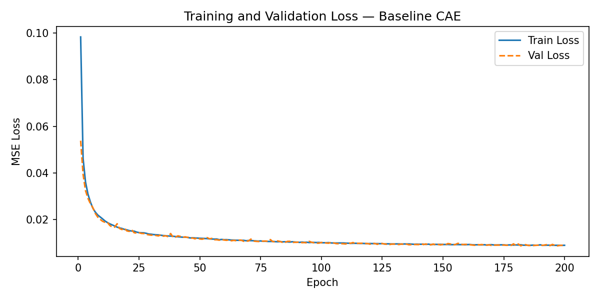
Figure 3. Training and validation loss curves for the baseline model (Adam, latent=128, 10×10 mask).
The baseline model converges smoothly, with the loss declining steeply during the first ~100 epochs before plateauing around epoch 170. The training and validation curves track each other closely throughout, indicating that the model is generalising rather than memorising the training set.
Test set MSE: 0.008868 (full 10,000-image test set).
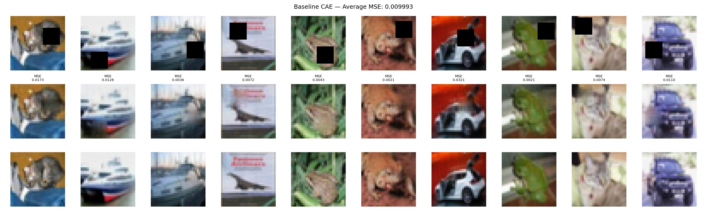
Figure 4. Predicted reconstructions vs. ground-truth images for the baseline model.
Visually, the model successfully recovers the coarse structure of occluded regions in most cases. However, reconstructed patches are noticeably smoother than the surrounding image — sharp edges and fine textures (e.g., fur, feathers) are replaced with averaged colour values. This is a direct consequence of the MSE objective, which minimises expected squared error by predicting the mean of all plausible completions, and is explored further in Section 3.2.
2.2 Optimizer Comparison
All three experiments in this section use identical hyperparameters (latent=128, 10×10 mask, 200 epochs, batch size 256), differing only in the optimizer. Note that Adam and RMSprop use a learning rate of 0.001, while SGD uses 0.01 — a higher starting rate that is conventional for SGD, which lacks adaptive per-parameter scaling.
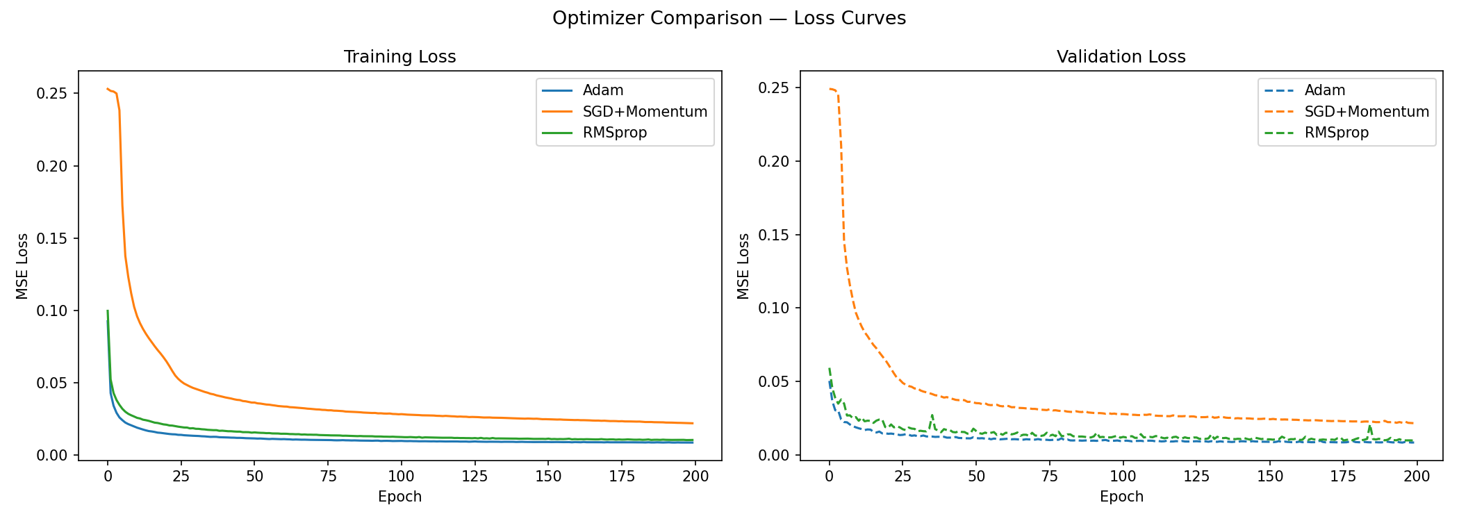
Figure 5. Training and validation loss curves for Adam, RMSprop, and SGD+Momentum.
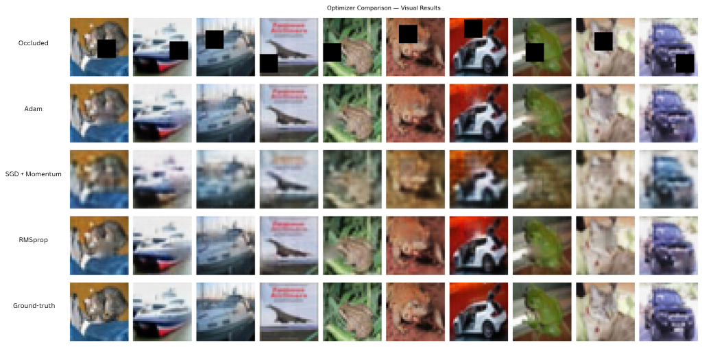
Figure 6. Predicted vs. ground-truth reconstructions for each optimizer.
| Optimizer | Final Test MSE | Notes |
|---|---|---|
| Adam | 0.008693 | Fastest convergence; lowest MSE. |
| RMSprop | 0.009822 | Stable training; slightly higher MSE than Adam. |
| SGD + Momentum | 0.021994 | Slow convergence; visibly blurred outputs. |
Interpretation. Adam achieves the lowest MSE and reaches a stable loss within roughly the first 75 epochs. Both Adam and RMSprop adapt their per-parameter learning rates based on gradient history, which accelerates convergence on the non-uniform loss landscape of an autoencoder. The difference between them (0.008693 vs. 0.009822, a gap of ~0.001) is small enough that a single run cannot definitively establish Adam’s superiority — both are reasonable choices.
SGD with momentum tells a clearer story: its MSE of 0.021994 is approximately 2.5× higher than Adam’s, and the visual outputs confirm noticeably blurred reconstructions. For a 32×32 image where individual pixel values matter, a fixed global learning rate with simple momentum is insufficient to navigate the high-dimensional loss landscape that adaptive methods handle naturally. This gap is large enough to be meaningful even with a single run.
2.3 Impact of Latent Dimensionality
The latent space is the bottleneck through which all image information must pass. Too small and the model cannot store enough information to reconstruct faithfully; too large and the model no longer needs to compress, risking simple memorisation.
An important upper bound: CIFAR-10 images are 32×32×3 = 3,072 values. After the encoder’s three stride-2 layers, the spatial map is 4×4. A latent channel count of C produces a latent tensor of C × 4 × 4 = 16C values. To remain a genuine compression, 16C must be less than 3,072, i.e., C < 192. The maximum tested value of C = 256 (4,096 latent values) slightly exceeds this bound and is included to illustrate the upper boundary of useful compression.
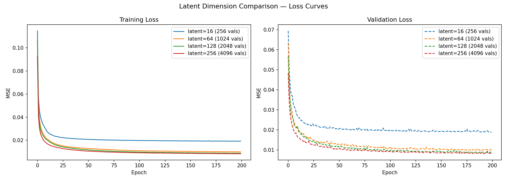
Figure 7. Training and validation loss for latent channel counts of 16, 64, 128, and 256.
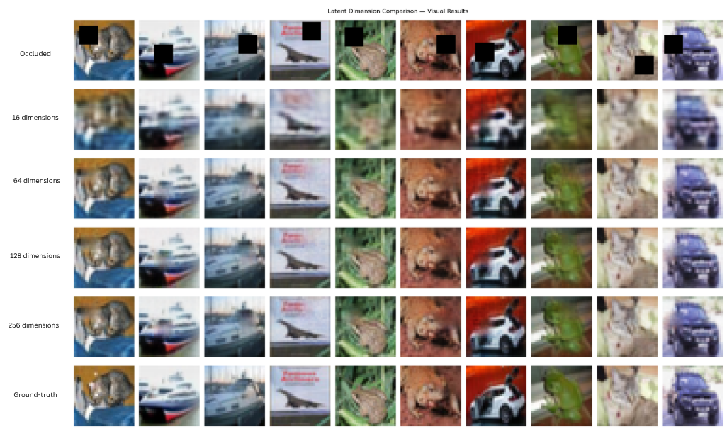
Figure 8. Predicted vs. ground-truth reconstructions for each latent dimension.
| Latent Channels | Latent Size | Final Test MSE | Notes |
|---|---|---|---|
| 16 | 256 | 0.019074 | Severe blurring; insufficient capacity. |
| 64 | 1,024 | 0.010753 | Significant improvement over 16. |
| 128 | 2,048 | 0.009221 | Good reconstruction; smaller gains. |
| 256 | 4,096 | 0.008309 | Best MSE; marginal gain over 128. |
Interpretation. The largest performance jump occurs between 16 and 64 channels: MSE drops by ~0.008 (45%). The improvement from 64 to 128 is smaller (~0.0015), and from 128 to 256 smaller still (~0.0009). This pattern of diminishing returns suggests that 128 channels captures most of the learnable structure in CIFAR-10 images at 32×32 resolution, and further capacity offers minimal benefit.
At C = 16, the model must compress 3,072 pixel values into just 256 latent values — a 12× reduction. The resulting outputs are visibly over-smoothed: the bottleneck is so tight that distinct textures are averaged away. At C = 256, the latent space (4,096 values) slightly exceeds the input dimensionality (3,072), which appears in Figure 7 as a wider train/validation gap — a sign that the model is beginning to memorise rather than compress. The 128-channel model sits comfortably between these extremes and is used as the baseline throughout.
2.4 Masking Strategy
To test whether training with more varied occlusion patterns improves robustness, two alternative masking strategies were compared against the baseline 10×10 square mask. All three strategies use the same total training budget (200 epochs, Adam, latent=128).
Importantly, all three strategies cover the same total pixel area of 100 pixels (~9.8% of the 32×32 image):
| Strategy | Configuration | Occluded Pixels | % of 32×32 Image |
|---|---|---|---|
| 10×10 square | 1 × 10×10 | 100 | ~9.8% |
| Random-size squares | Variable size | Variable | Variable |
| Multiple small masks | 4 × 5×5 | 100 | ~9.8% |
Because the baseline and multiple-mask strategies cover exactly the same total area, any performance difference between them is attributable to the spatial distribution of the mask, not to occlusion difficulty. The random-size strategy is an exception — because its mask size varies, total occluded area is not fixed, which must be kept in mind when interpreting its results.
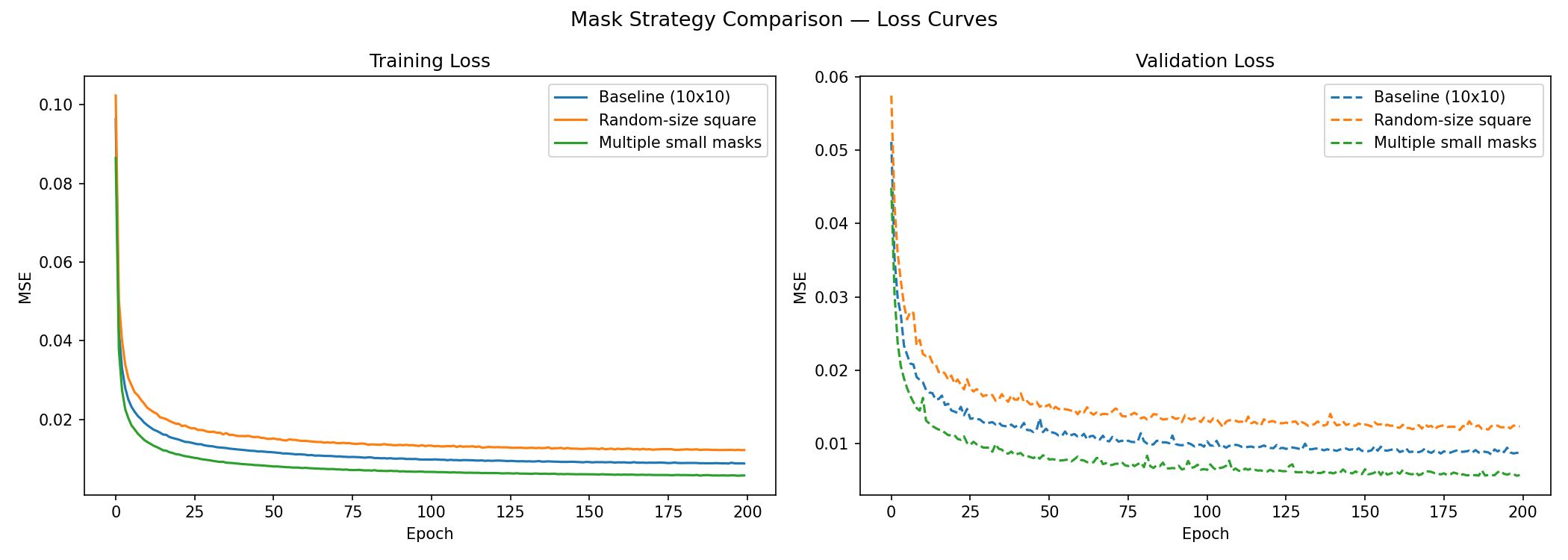
Figure 9. Training and validation loss for different masking strategies.
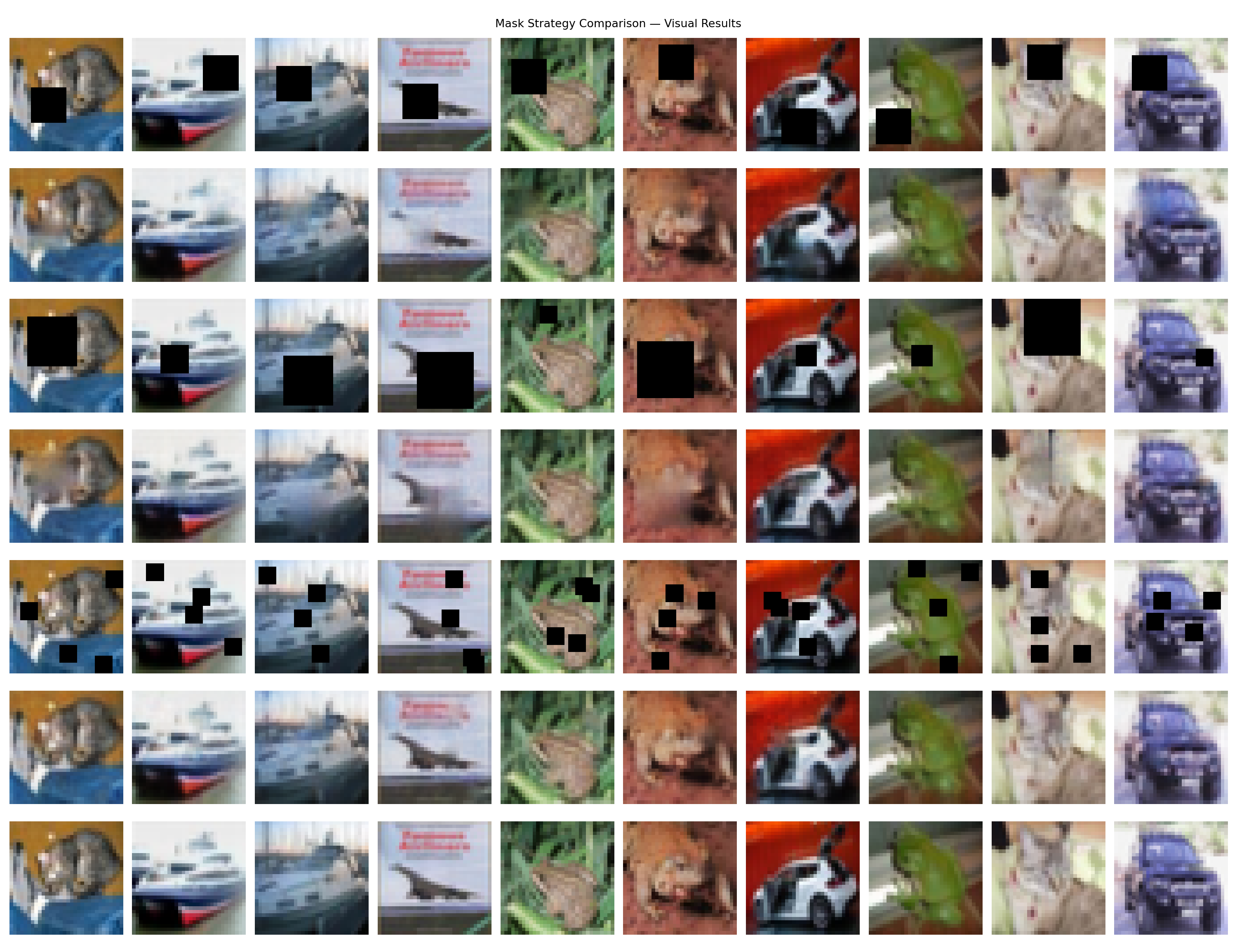
Figure 10. Predicted vs. ground-truth reconstructions for each masking strategy.
| Masking Strategy | Final Test MSE | Notes |
|---|---|---|
| 10×10 square | 0.008946 | Moderate; visible but contained artefact edges. |
| Random-size squares | 0.012345 | Highest MSE; struggles with variable-area occlusions. |
| Multiple squares | 0.005751 | Lowest MSE; nearly seamless reconstructions. |
Interpretation. The multiple-small-mask model achieves the best quantitative and visual result — despite covering exactly the same total area as the baseline. This makes the comparison particularly clean: the improvement cannot be attributed to masking less of the image. Training on four spatially scattered 5×5 masks instead of one 10×10 mask appears to encourage the model to learn spatial context from a wider neighbourhood, as the model must attend to diverse surroundings to fill in each small patch rather than relying on a single adjacent edge.
The random-size square model performs worst. Its variable masking area means that training difficulty is highly inconsistent — occasionally the model encounters a near-fully-occluded image and cannot learn a reliable strategy. The resulting average loss is dragged upward by these hard cases.
Testing the baseline on multiple masks. To measure how sensitive the baseline (trained on a single 10×10 mask) is to increased occlusion at test time, the number of applied masks was increased progressively:
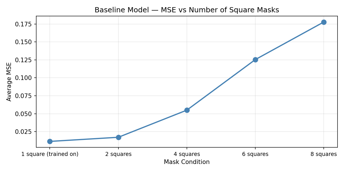
Figure 11. Baseline model test MSE as the number of 10×10 test-time masks increases from 1 to N.
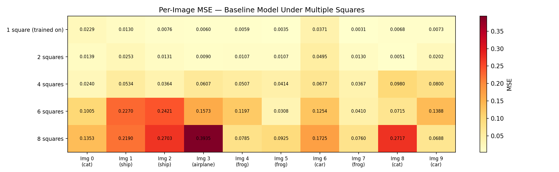
Figure 12. Per-image MSE heatmap across all 10 test images as mask count increases. Each row is one image; each column is a mask count.
Performance degrades consistently across all 10 test images as mask count increases (Figure 12), ruling out the possibility that degradation was caused by a particularly hard image category. The decline is driven by increased total occlusion — as more pixels are hidden, the model has less surrounding context available for inference. This is expected behaviour and demonstrates that a single-mask model is a poor fit for real-world inpainting, where corruption patterns are irregular and variable.
3. Limitations
3.1 Dataset Resolution
CIFAR-10 images are 32×32 pixels. At this resolution, each image contains at most 1,024 pixels per channel, which limits both what the model can learn and what can meaningfully be reconstructed. When a 10×10 region is missing, the model must infer ~100 pixels from at most ~924 surrounding pixels — many of which may themselves be from a different semantic region (e.g., background sky vs. foreground object). Higher-resolution images would provide more local context around each masked region, giving the model more information to work with and likely resulting in sharper reconstructions.
3.2 The MSE Blurring Problem
MSE minimises the expected squared pixel error. When a masked patch could be completed in multiple plausible ways (e.g., the texture of a bird’s feathers could plausibly continue in several directions), the optimal MSE prediction is the average of all those possibilities — which, visually, produces a blurred patch. The model is not making a mistake; it is being mathematically optimal under the wrong objective. This is a known fundamental limitation of pixel-wise regression losses in generative tasks, and it motivates the combined MAE + perceptual loss used in Part B.
4. Proposed Improvements
4.1 Higher-Resolution Dataset
Replacing CIFAR-10 with STL-10 would address the resolution bottleneck. STL-10 contains 96×96 colour images across 10 similar classes, with 500 training images per class and 100,000 unlabelled images for unsupervised pre-training. The 9× increase in pixels per image provides substantially more context around each masked region and gives the model more structure to encode in the latent space.
4.2 Perceptual and MAE Loss Functions
Two loss functions directly address the blurring problem identified in Section 3.2:
Mean Absolute Error (L1 loss): Unlike MSE, MAE does not square the error, so it does not disproportionately penalise large differences. In practice, MAE tends to produce reconstructions with sharper edges because it tolerates small errors more evenly across the image.
Perceptual Loss: Instead of comparing images pixel-by-pixel, perceptual loss passes both the reconstructed and ground-truth images through a pretrained feature extractor and minimises the difference between intermediate feature maps. Because these features encode edges, textures, and object parts rather than individual pixels, the model is guided toward outputs that look realistic to the human visual system. This combination is adopted and evaluated in Part B.
Part B: Vision Transformer
1. Motivation from CAE Results
Part A established two clear lessons:
MSE is insufficient as a sole loss function. It reliably recovers global structure but produces blurred reconstructions wherever fine texture must be inferred.
Local convolutions limit spatial reasoning. The CAE’s receptive field grows only through stacking layers. When a masked region has no close neighbours that share its texture, the model has limited ability to draw on distant context.
These two observations motivate the use of a Vision Transformer and a combined MAE + perceptual loss for Part B.
2. Why a Vision Transformer?
Convolutional layers process local neighbourhoods — each output pixel depends on a small spatial window of the input. This means global context must propagate through many layers. Vision Transformers instead process an image as a sequence of patches, and self-attention computes relationships between every pair of patches in a single operation — regardless of spatial distance. This gives the model global context from the very first layer, which is particularly valuable for inpainting: a masked region can be informed by similar textures anywhere else in the image, not just its immediate neighbours.
The trade-off is that Transformers lack the spatial inductive biases of CNNs and therefore require more data and compute to achieve equivalent performance. This limitation is acknowledged in Section 7.
3. Dataset and Masking Strategy
Due to compute and timeline constraints, the Oxford-IIIT Pet Dataset was used — approximately 7,300 images of 37 breeds of cats and dogs. This provides sufficient variety for learning texture and structure while remaining tractable to train.
Informed by the CAE finding that multiple small masks produce better generalisation, the ViT uses the multiple square masks strategy throughout training. The masking configuration was varied across training phases, as described in Section 5.
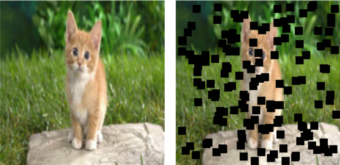
Figure 13. Example input: 150 masks of size 11×11 applied to a 224×224 image (~36% occluded).
4. Model Architecture
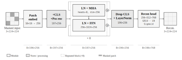
Figure 14. Vision Transformer architecture used for inpainting.
The pipeline proceeds as follows:
Patch Embedding. The 224×224 input image is divided into a grid of non-overlapping 16×16 patches (14×14 = 196 patches total). Each patch is linearly projected into a 256-dimensional embedding vector. A learnable positional encoding is added to each embedding so the model knows where each patch originally came from — without this, the self-attention mechanism is permutation-invariant and cannot distinguish spatial arrangement.
Transformer Encoder. Eight transformer blocks process the sequence of 196 patch embeddings. Each block contains:
- Multi-Head Self-Attention (8 heads): Computes attention weights between all 196×196 patch pairs, allowing any patch to directly draw information from any other patch in the image.
- Feed-Forward MLP: Applies a two-layer non-linear transformation to each patch embedding independently, refining the features extracted by attention.
- Residual connections and layer normalisation around each sub-component, which stabilise gradient flow through the 8 stacked blocks.
Reconstruction Head. A two-layer MLP maps each patch embedding back to pixel values. Concretely: Linear(256 → 512) → GELU → LayerNorm → Linear(512 → 16×16×3 = 768), followed by a Sigmoid activation. Outputs are clamped to [0, 1]. The non-linear head gives the model more expressive power in the final reconstruction step compared to a single linear projection.
Loss function. A weighted combination of MAE and Perceptual Loss is used:
\[L_{\text{total}} = \lambda_{\text{MAE}} \cdot L_{\text{MAE}} + \lambda_{\text{Perceptual}} \cdot L_{\text{Perceptual}}\]where:
\[L_{\text{MAE}} = \frac{1}{N} \sum_{i=1}^{N} |x_i - \hat{x}_i|\] \[L_{\text{Perceptual}} = \sum_j \frac{1}{C_j H_j W_j} \|\phi_j(x) - \phi_j(\hat{x})\|_1\]Here \(\phi_j\) denotes the feature maps extracted from the first 16 layers of a pretrained VGG-16 network, with inputs re-normalised to ImageNet mean and standard deviation before being passed through VGG. The L1 norm is used for the feature comparison. Comparing reconstructions in feature space penalises deviations in texture and structure rather than raw pixel values.
Training infrastructure. Mixed Precision Training (PyTorch AMP with GradScaler) was used throughout to reduce memory usage and accelerate training.
Baseline ViT hyperparameters (Epoch 1):
| Hyperparameter | Value |
|---|---|
| Loss Function | MAE + Perceptual |
| Input Resolution | 224×224 |
| Optimizer | AdamW |
| Patch Size | 16×16 |
| Embedding Dim | 256 |
| Transformer Blocks | 8 |
| Attention Heads | 8 |
| Dropout | 0.1 |
| Learning Rate | 0.001 (initial) |
| Batch Size | 64 |
| Trainable Parameters | 8,671,744 |
AdamW vs. Adam. AdamW differs from standard Adam in how weight decay is applied: rather than incorporating weight decay into the gradient update (which interacts with the adaptive learning rate scaling), AdamW applies it directly to the parameters as a separate step. This decoupled formulation is more theoretically principled and empirically tends to generalise better, particularly for Transformer models — making it a natural choice here.
The architectural choices — 8 blocks, 8 heads, 256 dimensions — were selected to balance model capacity with the available dataset size (~7,300 images). A larger model risks overfitting on this relatively small dataset.
5. Training Strategy
Because the dataset is small relative to the model’s capacity, and because the loss function was adjusted throughout training, a fixed hyperparameter schedule was not feasible from the outset. Training was divided into seven phases, each targeting a specific failure mode identified during inspection of validation outputs.
Reproducibility note. The manual phase transitions described below represent the primary reproducibility limitation of this experiment. The epoch numbers at which shifts occur and the specific weight values chosen were determined by visual inspection during training. In addition, the masking configuration was updated via the training scheduler per phase, but the mask application function used default values of
num_masks=150, mask_size=11throughout; the phase-specific mask parameters describe the intended schedule. Automated loss-weighting methods (GradNorm, SoftAdapt, Uncertainty Weighting) are discussed in Section 7.2 as more principled alternatives.
The dataset was split 80/20 into training and test sets, with no separate validation split. Loss curves therefore show train vs. test loss throughout.
Phase 1: Foundation (Epochs 1–20)
| LR | Mask Size | Num Masks | \(\lambda_{\text{MAE}}\) | \(\lambda_{\text{Perceptual}}\) |
|---|---|---|---|---|
| 0.001 | 9×9 | 80 | 1.0 | 0.0 |
Training begins with pure MAE loss (\(\lambda_{\text{Perceptual}}\) = 0.0). At initialisation, the model produces near-random outputs. Applying perceptual loss at this stage — confirmed in a preliminary test shown below — causes VGG-16 to detect high-frequency noise as a large feature mismatch, producing extreme gradient magnitudes and immediate instability. Starting with MAE alone allows the model to first learn broad image structure before any perceptual penalty is introduced.
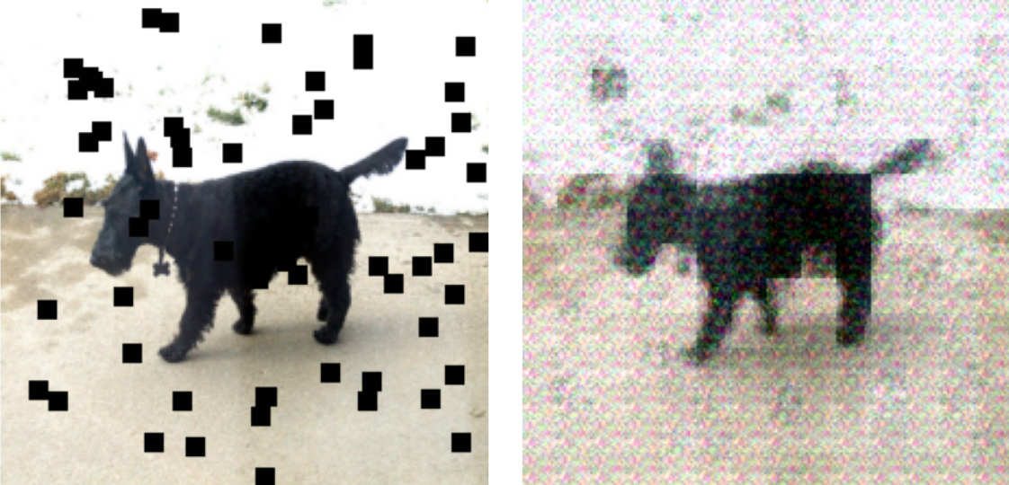
Figure 15. Output when perceptual loss is introduced too early ($$\lambda_{\text{MAE}}$$=0.7, $$\lambda_{\text{Perceptual}}$$=0.3 at epoch 20). The model produces RGB noise that persists throughout training.
By epoch 20, outputs are blurry but structurally recognisable.
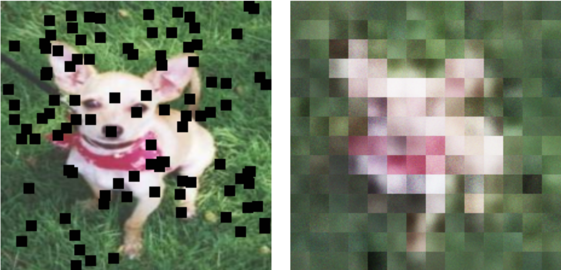
Figure 16. Reconstruction at epoch 20 ($$\lambda_{\text{MAE}}$$=1.0, $$\lambda_{\text{Perceptual}}$$=0.0). Blurry but structurally correct.
Phase 2: Introducing Perceptual Loss Gradually (Epochs 21–40)
| LR | Mask Size | Num Masks | \(\lambda_{\text{MAE}}\) | \(\lambda_{\text{Perceptual}}\) |
|---|---|---|---|---|
| 0.0001 | 9×9 | 80 | 1.0→0.8 | 0.0→0.2 |
With the model producing coherent coarse reconstructions, perceptual loss is introduced. An initial attempt to jump directly from (1.0, 0.0) to (0.8, 0.2) caused an abrupt spike in loss magnitude — perceptual loss operates on VGG-16 feature activations whose numerical scale is very different from per-pixel MAE.
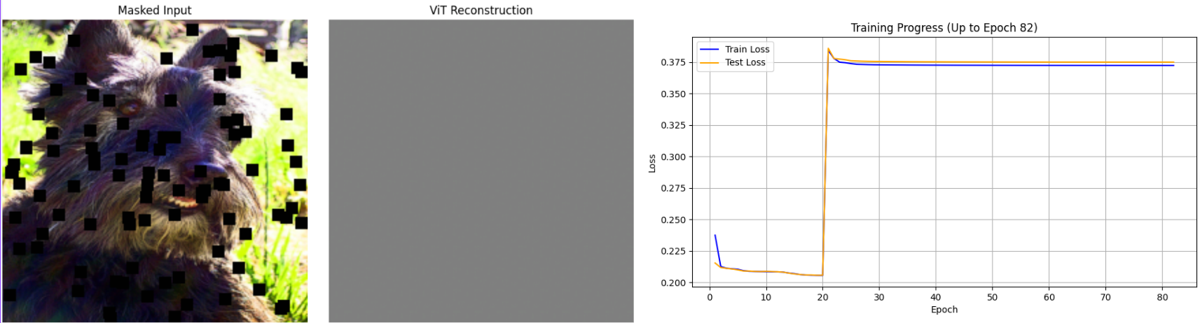
Figure 17. Gradient explosion caused by an abrupt weight shift. Left: loss spike in the training plot. Right: output degenerates to a uniform grey image.
Two countermeasures were applied to resolve this:
- Linear interpolation of the weights across epochs 21–39 (from (1.0, 0.0) to (0.8, 0.2)), introducing the perceptual signal at a rate the optimiser could adapt to.
- Gradient clipping (
torch.nn.utils.clip_grad_norm_,max_norm=1.0), which hard-limits the gradient magnitude regardless of the loss scale, providing a safety net against future spikes.
The learning rate scheduler is disabled during this phase because the validation loss temporarily rises — not because the model is getting worse, but because the objective function itself is changing.
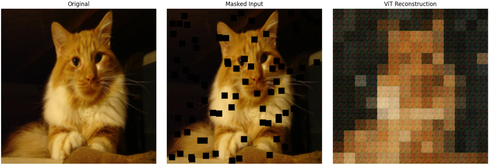
Figure 18. Reconstruction at epoch 40. The transition was handled without gradient explosion. Residual RGB noise is visible but manageable.
Phase 3: Consolidation (Epochs 41–135)
| LR | Mask Size | Num Masks | \(\lambda_{\text{MAE}}\) | \(\lambda_{\text{Perceptual}}\) |
|---|---|---|---|---|
| 0.0001 | 9×9 | 80 | 0.8 | 0.2 |
With the loss function stabilised, this phase allows the model to train at fixed weights. At epoch 110, the learning rate was increased from 0.0001 to 0.0002 to accelerate convergence after a visible plateau. By epoch 135, reconstructions show notably more defined features, though a characteristic mosaic artefact is visible — patch boundaries appear as block discontinuities in the output.
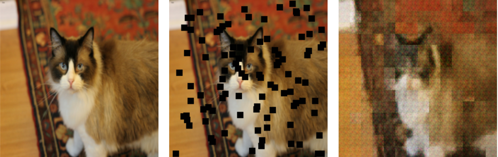
Figure 19. Reconstruction at epoch 135. Structure is well-recovered; patch-boundary mosaic artefact is evident.
The mosaic artefact arises because the model produces one colour prediction per 16×16 patch, and adjacent patches can converge to slightly different average colours. This is a known ViT inpainting limitation discussed further in Section 7.3.
Phase 4: Reducing Mosaic Artefacts (Epochs 136–200)
| LR | Mask Size | Num Masks | \(\lambda_{\text{MAE}}\) | \(\lambda_{\text{Perceptual}}\) |
|---|---|---|---|---|
| 0.0004 | 9×9 | 80 | 0.6 | 0.4 |
The perceptual loss weight is increased to 0.4 and the learning rate to 0.0004. VGG-16 feature maps capture edge structure at multiple scales, so increasing \(\lambda_{\text{Perceptual}}\) explicitly penalises the block discontinuities at patch boundaries.
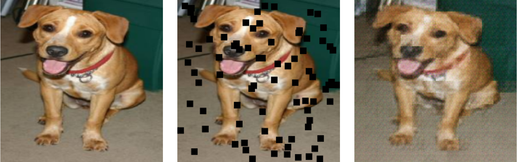
Figure 20. Reconstruction at epoch 200. Mosaic artefacts are significantly reduced; edge continuity is improved.
Phase 5: High-Difficulty Training (Epochs 201–270)
| LR | Mask Size | Num Masks | \(\lambda_{\text{MAE}}\) | \(\lambda_{\text{Perceptual}}\) |
|---|---|---|---|---|
| 0.0004 | 11×11 | 150 | 0.6 | 0.4 |
Both mask size and count are increased, raising total occlusion from approximately 13% to ~36% of the image area. The loss weights remain fixed, ensuring that the edge preservation improvement from Phase 4 is retained while the model adapts to a harder inpainting task.
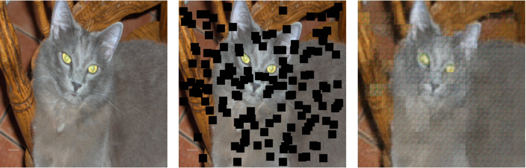
Figure 21. Reconstruction at epoch 270 (150 masks, size 11×11, ~36% occlusion). Quality is well-maintained despite increased difficulty.
Phase 6: Pushing to ~48% Occlusion (Epochs 271–350)
| LR | Mask Size | Num Masks | \(\lambda_{\text{MAE}}\) | \(\lambda_{\text{Perceptual}}\) |
|---|---|---|---|---|
| 0.0004 | 11×11 | 200 | 0.5 | 0.5 |
Mask count is raised to 200, covering approximately 200 × 121 / (224²) ≈ 48% of the image. The perceptual weight is increased to 0.5, equalising its influence with MAE. Despite another brief loss spike at the phase transition, training stabilises and reconstruction quality is maintained.
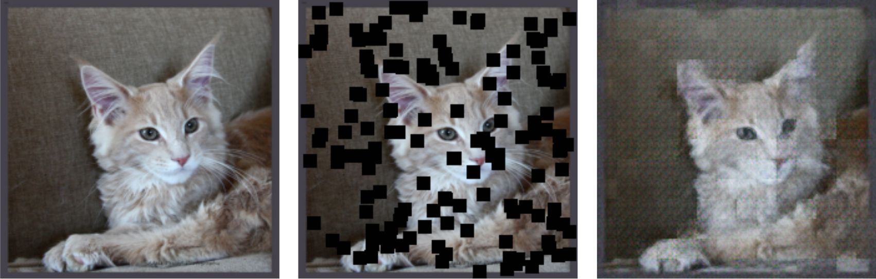
Figure 22. Reconstruction at epoch 350 (200 masks, size 11×11, ~48% occlusion).
Phase 7: Dynamic Masking (Epochs 351–400)
| LR | Mask Size | Num Masks | \(\lambda_{\text{MAE}}\) | \(\lambda_{\text{Perceptual}}\) |
|---|---|---|---|---|
| 0.0004 | 9×9 – 12×12 (random) | 175–300 (random) | 0.5 | 0.5 |
In the final phase, both mask size and count are randomised per batch across the stated ranges, rather than fixed. This prevents the model from adapting to a specific occlusion pattern and forces it to develop a more general inpainting policy. Mask counts of 175–300 correspond to roughly 42–69% of the image area.
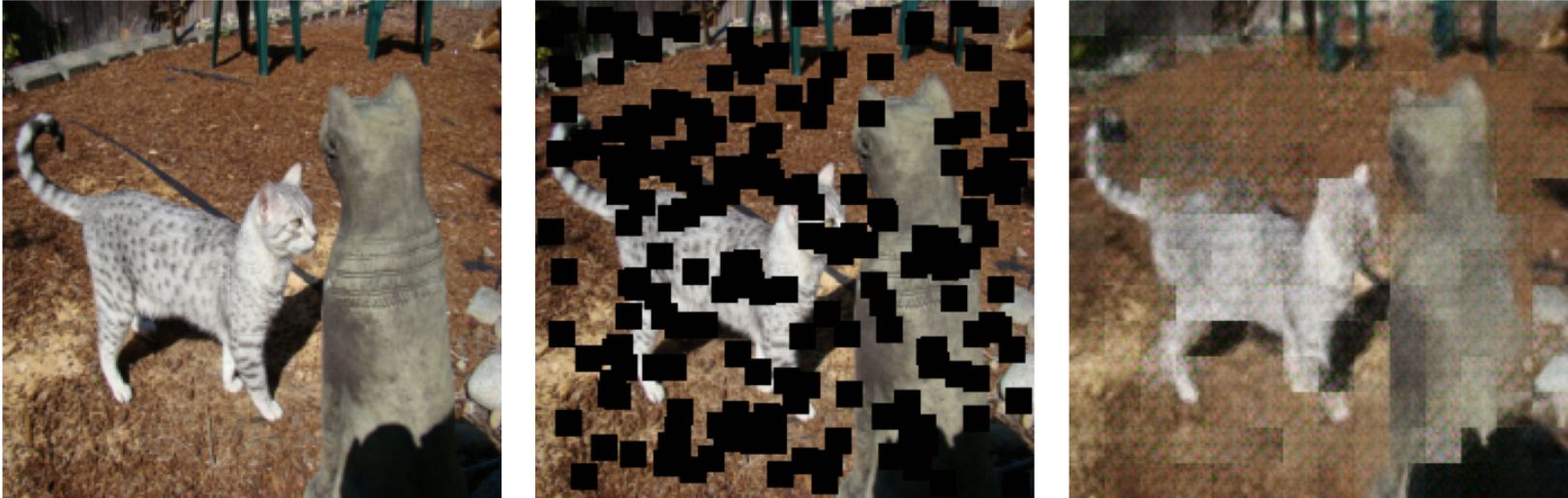
Figure 23. Reconstruction at epoch 400 (200 masks, size 12×12). High occlusion is handled with reasonable fidelity.
6. Results and Discussion
6.1 Full Training Progress
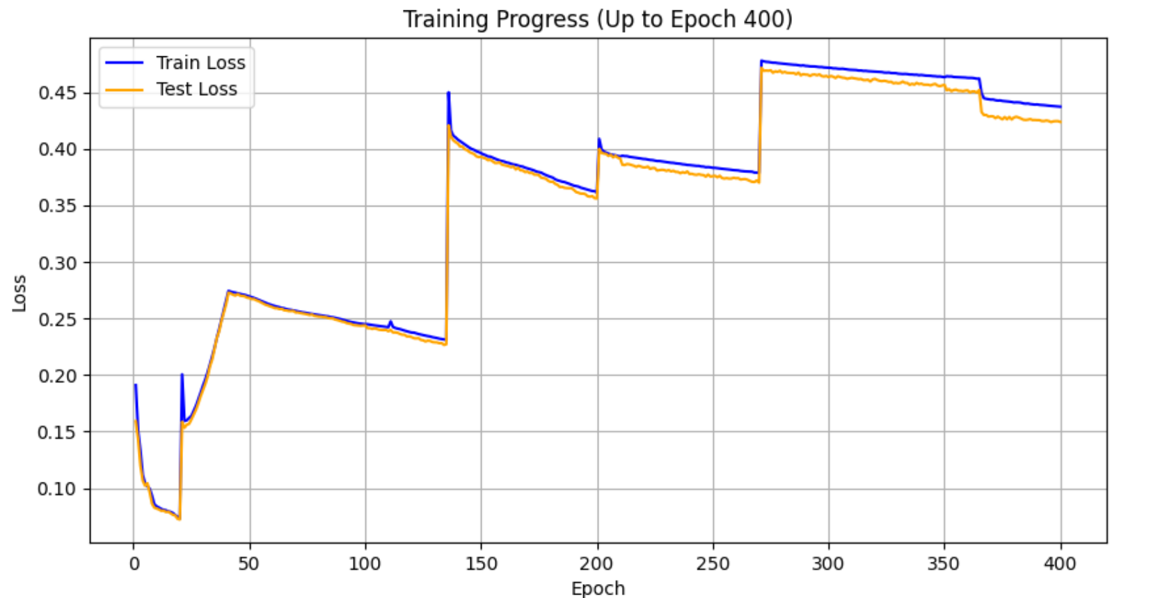
Figure 24. Training and test loss across all 400 epochs. Phase transitions are visible as loss spikes, each followed by a return to a lower baseline than before.
The loss curve does not follow the clean monotonic descent typical of a fixed-objective experiment. Each phase transition introduces a temporary spike — either because the objective changes (weight shifts) or because the task difficulty increases (more masks). That the loss consistently returns to a lower baseline after each spike confirms that the model is improving across phases. Comparing loss values numerically across phases is not meaningful because the objective function changes between phases; progress is best assessed visually (Figures 16–23) and through the generalisation experiments below.
6.2 Generalisation
Test 1: Unseen images from the training class distribution. Images from outside the training set were masked with 150–250 occlusions of size 11×11.
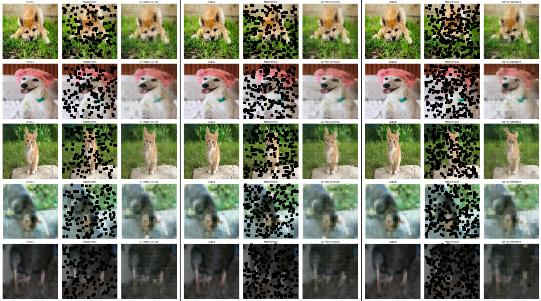
Figure 25. Left: 150 masks. Centre: 200 masks. Right: 250 masks. Test images are drawn from outside the training set. Reconstructions remain coherent across increasing occlusion levels.
Test 2: Entirely unseen object categories. The model was tested on images of ships and boats — categories absent from the Oxford-IIIT Pet Dataset.
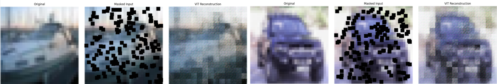
Figure 26. Inpainting results on ships and boats — categories unseen during training. Overall shape and colour distribution are preserved, though reconstructions are blurrier than for animal images.
Interpretation. The model performs well on unseen images from similar categories (Figure 25), as expected. The more informative finding is Figure 26: the model produces recognisable reconstructions of ships and boats despite training exclusively on animals. This suggests the model has learned general inpainting priors — filling based on colour gradients, edge continuation, and structural continuity — rather than memorising animal-specific textures. Performance is lower than for animals, as expected, but the outputs are not random or degenerate.
That said, these observations are based on a small number of test images. A rigorous generalisation claim would require systematic evaluation on a labelled out-of-distribution dataset with quantitative metrics. The results here should be treated as encouraging indicative evidence, not proof.
7. Limitations and Future Work
7.1 Data Hunger and Dataset Size
Vision Transformers lack the inductive biases of convolutional networks — they do not assume nearby pixels are more related than distant ones, nor that useful features repeat across the image. These assumptions, baked into CNNs, are what make CNNs data-efficient. Without them, ViTs need substantially more data to learn equivalent representations.
The Oxford-IIIT Pet Dataset’s ~7,300 images are far below what a ViT would ideally train on. The extensive manual training schedule in Section 5 — seven phases, repeated learning rate adjustments, and careful loss weight tuning — is in large part a workaround for this data limitation. With a larger dataset such as ImageNet or CelebA-HQ, the model would likely converge to better representations with a simpler, fixed training schedule.
7.2 Manual Loss Weight Scheduling
The phase-based approach to adjusting \(\lambda_{\text{MAE}}\) and \(\lambda_{\text{Perceptual}}\) was determined by visual inspection at runtime. This introduces two problems: the schedule is not fully reproducible, and it is sensitive to the particular run’s behaviour. Several principled alternatives exist:
- Uncertainty Weighting (Kendall et al., 2018): Models the homoscedastic uncertainty of each loss component as a learnable parameter, automatically down-weighting objectives that are already well-minimised.
- GradNorm (Chen et al., 2018): Dynamically adjusts loss weights by normalising gradient magnitudes across objectives, ensuring all losses train at comparable rates.
- SoftAdapt (Heydari et al., 2019): Shifts weights toward objectives that are currently harder to minimise, based on their recent rate of change.
Any of these methods would replace the manual schedule with a principled, reproducible mechanism, and represents the most important improvement to pursue in follow-up work.
7.3 Patch Boundary Artefacts
The mosaic artefact observed in Phases 3–4 is a structural consequence of the 16×16 patch grid: each patch embedding is decoded to a single 16×16 tile, and if adjacent tiles converge to different mean colours, the boundary is visible. Mitigation strategies include:
- Overlapping patches with averaging at boundaries (at higher computational cost).
- Convolutional upsampling in the reconstruction head, which smooths across patch boundaries.
- Smaller patch sizes (e.g., 8×8), which produce finer-grained predictions at the cost of a longer sequence (784 patches vs. 196) and higher memory requirements.
8. Conclusion
This project explored image inpainting across two architectures: a Convolutional Autoencoder on CIFAR-10 and a Vision Transformer on the Oxford-IIIT Pet Dataset.
The CAE experiments established clear conclusions: Adam outperforms SGD significantly; latent dimensionality yields diminishing returns beyond 128 channels; and training with multiple small masks (same total area, scattered distribution) produces better inpainting than a single large mask. These findings are consistent with established understanding of adaptive optimisers and information bottlenecks.
The ViT experiments are harder to summarise cleanly because the training process was necessarily irregular. The model does learn to inpaint, and shows surprising generalisation to unseen object categories. But the process required constant manual intervention — a sign that the model was being coaxed to learn rather than converging naturally. This is primarily a consequence of the small dataset and shifting loss function, and is honestly acknowledged as a limitation rather than obscured.
The central methodological lesson across both parts is that the loss function defines what the model learns to value. MSE produces structurally correct but blurred outputs because blurring is the optimal MSE strategy when texture is ambiguous. A combined MAE + perceptual loss redirects the model toward outputs that look plausible to a feature extractor calibrated on natural images — and the improvement in visual quality between Figures 4 and 25 reflects exactly this shift in objective.
References
- Krizhevsky, A. (2009). Learning Multiple Layers of Features from Tiny Images. Technical Report.
- Kingma, D.P. and Ba, J. (2014). Adam: A Method for Stochastic Optimization. arXiv:1412.6980.
- Loshchilov, I. and Hutter, F. (2019). Decoupled Weight Decay Regularization. ICLR 2019.
- Qian, N. (1999). On the Momentum Term in Gradient Descent Learning Algorithms. Neural Networks.
- Johnson, J., Alahi, A. and Fei-Fei, L. (2016). Perceptual Losses for Real-Time Style Transfer and Super-Resolution. ECCV 2016.
- Dosovitskiy, A. et al. (2021). An Image is Worth 16×16 Words: Transformers for Image Recognition at Scale. ICLR 2021.
- Naseer, M. et al. (2021). Intriguing Properties of Vision Transformers. NeurIPS 2021.
- Kendall, A., Gal, Y. and Cipolla, R. (2018). Multi-Task Learning Using Uncertainty to Weigh Losses for Scene Geometry and Semantics. CVPR 2018.
- Chen, Z. et al. (2018). GradNorm: Gradient Normalization for Adaptive Loss Balancing in Deep Multitask Networks. ICML 2018.
- Heydari, A.A., Thompson, C.A. and Mehmood, A. (2019). SoftAdapt: Techniques for Adaptive Loss Weighting of Neural Networks with Multi-Part Loss Functions. arXiv:1912.12355.