
Learning Continuous LiDAR Navigation in a Randomised Cone Maze
Published:
Introduction
This project asks whether a small holonomic robot can learn to cross a cluttered corridor from sensor data alone. The vehicle is placed at one end of a 7.2-metre corridor facing a randomly generated field of obstacles and must reach the far side without touching anything. Because the layout is regenerated for every episode, a trajectory cannot be memorised; the controller has to acquire a general policy for moving through confined spaces.
The result is a controller that succeeds on 83.7% of 300 medium-difficulty episodes (251/300), a figure that was also independently re-evaluated at 83.0% (249/300). It was produced by a four-stage pipeline: a hand-written expert controller, behaviour cloning from that expert, three rounds of dataset aggregation (DAgger), and a conservative teacher-anchored fine-tuning stage using proximal policy optimisation (PPO). The champion checkpoint is the one at 132,400 timesteps
Two properties of the platform determine the form of any viable solution:
- The vehicle is holonomic. Forward, lateral and rotational motion are commanded independently, so it can translate past an obstacle without first turning to face it — a real advantage in a narrow gap. It also means three continuous commands must be coordinated at once, which makes a discrete action set a poor representation of the available behaviour.
- Perception is a single planar LiDAR scan of thirty-six range measurements, plus a small amount of state information including the goal direction. There is no map, no camera, and no temporal history. Any behaviour that requires memory of previous observations has to be encoded in the policy itself.
Like every simulation work, a substantial part of the work was tuning the simulation environment to allow for smooth training. For example, the expert controller went from 20% to 85% success rate just from correcting a threshold in the simulation environment, not from any change to the learner. Part III documents that work, because the diagnosis was more transferable than the result.
A note on scope. This page covers the supervised stage of the project: the expert, imitation, and the PPO extension that produced the champion. A later stage investigating whether the same task could be learned without expert supervision is summarised in a single line at the end.
Part I: Task and Platform
1. The simulation environment
Everything was developed and evaluated in simulation, on a stack of ROS 2 Jazzy, Gazebo Harmonic, Gymnasium, Stable-Baselines3 and PyTorch. The bridge between simulator and learner is ros_gz_bridge, carrying /scan, /odom, /cmd_vel and /clock.
The environment runs a 20 Hz LiDAR and waits for one fresh scan and odometry update per action, giving a nominal decision interval of 0.05 s. An episode permits at most 800 decisions, about 40 seconds of simulated time. Actual odometry timestamp deltas are logged, because process load can make the real interval differ from the nominal one.
2. Observation space
The policy receives a 42-element float32 vector:
| Indices | Quantity | Normalisation | Purpose |
|---|---|---|---|
| 0–35 | Uniformly sampled 360° LiDAR rays | clipped to 10 m, divided by 10 | Local obstacle geometry |
| 36–37 | Unit vector toward the goal, in the robot body frame | $[-1, 1]$ | Goal direction stays observable while yaw is controllable |
| 38 | Goal distance | divided by 8 m, clipped to $[0, 1]$ | Remaining task scale |
| 39–41 | Previous applied action | $[-1, 1]$ | Makes the actuation history observable |
Two choices in that vector are deliberate. Rotating the goal vector into the body frame means the goal direction is unambiguous regardless of heading, which matters precisely because yaw is a free variable here. Including the previously applied command lets the policy account for the velocity filter, which brings the observation closer to Markovian.
Invalid ranges are handled conservatively: positive infinity becomes the maximum range, while NaN and negative infinity become unsafe zero-range readings before clipping. Thirty-six rays are compact, but they cannot guarantee detection of geometry that falls between sampled angles.
3. Action space and actuation
The policy emits a normalised triple
\[u_t = [u_x, u_y, u_\psi], \qquad u_i \in [-1, 1],\]mapped to body-frame velocity commands
\[v_x = 0.4\,u_x \;\text{m/s}, \qquad v_y = 0.4\,u_y \;\text{m/s}, \qquad \omega_z = 0.8\,u_\psi \;\text{rad/s}.\]Learned commands pass through a per-axis directional filter before reaching the actuators. It is deliberately asymmetric — a brake-fast, accelerate-smoothly filter rather than a symmetric low-pass — and each axis is treated differently depending on how the new request relates to the command currently applied:
| Case for axis $i$ | Applied command | Rationale |
|---|---|---|
| Requested reversal, $u_i \cdot a_{i,t-1} < 0$ | $a_{i,t} = 0$ | never cross through zero in a single control tick |
| Decreasing magnitude, $\lvert u_i \rvert \le \lvert a_{i,t-1} \rvert$ | $a_{i,t} = u_i$, applied immediately | braking and releasing an axis must not be delayed |
| Increasing magnitude | $a_{i,t} = a_{i,t-1} + \alpha\,(u_i - a_{i,t-1})$, $\alpha = 0.15$ | accelerate smoothly |
Only the third case is a low-pass filter, and it is the only one that involves $\alpha$. The consequence is that a command to stop, reverse, or ease off an axis reaches the actuators on the very next tick, while a command to push further is ramped in over several ticks. The platform’s brake-fast, accelerate-slowly asymmetry is therefore enforced in software rather than left for the policy to discover, and arbitrary diagonal and curved commands remain available.
4. Reward and termination
For a non-terminal transition the reward is
\[r_t = 5(x_t - x_{t-1}) - 0.0025 - 0.10\lVert a_t - a_{t-1}\rVert_2^2 - 0.002\lvert\omega_t\rvert - 0.05\frac{\max(0,\,0.45 - d_t)}{0.45} + r_{terminal}\]with $r_{terminal} = +20$ for success and $-40$ for collision or leaving the corridor.
| Term | Value | Rationale |
|---|---|---|
| Forward progress | $5\,\Delta x$ | Directly rewards movement toward the finish line |
| Step charge | 0.0025 | Equals the earlier 0.05-per-second cost at 20 decisions per second |
| Applied action change | $-0.10\lVert\Delta a\rVert^2$ | Discourages abrupt commands, but stays small enough to allow evasive manoeuvres |
| Yaw cost | $-0.002\lvert\omega\rvert$ | Discourages unnecessary spinning without forbidding rotation |
| Proximity cost | $-0.05$ inside 0.45 m | Begins well before the collision boundary, so pressure arrives early |
| Terminal | $+20$ / $-40$ | The failure cost exceeds the maximum plausible forward-progress reward |
On a collision or out-of-bounds transition, positive progress is clamped away, so a large terminal jump cannot offset the failure penalty. Episodes end on success, collision, or boundary violation, and truncate after 800 decisions:
| Event | Rule |
|---|---|
| Success | world $x$ reaches or exceeds 7.2 m, unless collision takes precedence |
| Collision | minimum of the sampled LiDAR scan is at or below the collision threshold |
| Out of bounds | $\lvert y\rvert \ge 2.15$ m |
| Time limit | 800 decisions reached |
The goal is a finish line, not a point at $(7.2, 0)$. That is why forward progress is the correct primary measure — a Euclidean distance-to-goal term would pull a perfectly valid trajectory toward the centre of the corridor for no reason.
Four different distances are in play at once, and their ordering is deliberate:
| Function | Distance |
|---|---|
| Collision termination | 0.15 m |
| DAgger safety intervention | 0.24 m |
| Expert movement clearance | 0.30 m |
| Reward proximity | 0.45 m |
Each margin fires before the next, so behavioural pressure builds up before any hard boundary is reached. Collapsing all four to the collision value would remove that graduated response entirely.
5. Maze generation
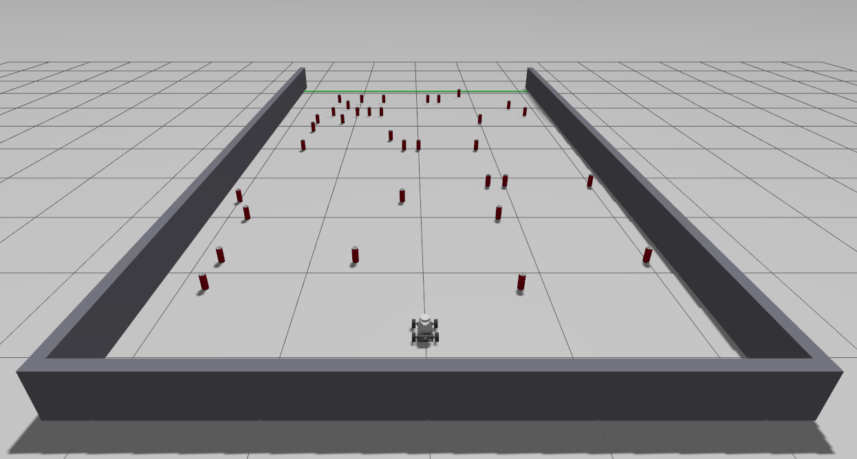
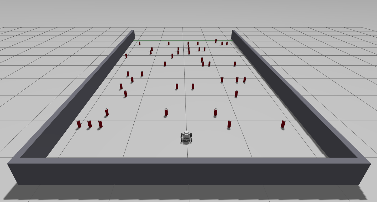
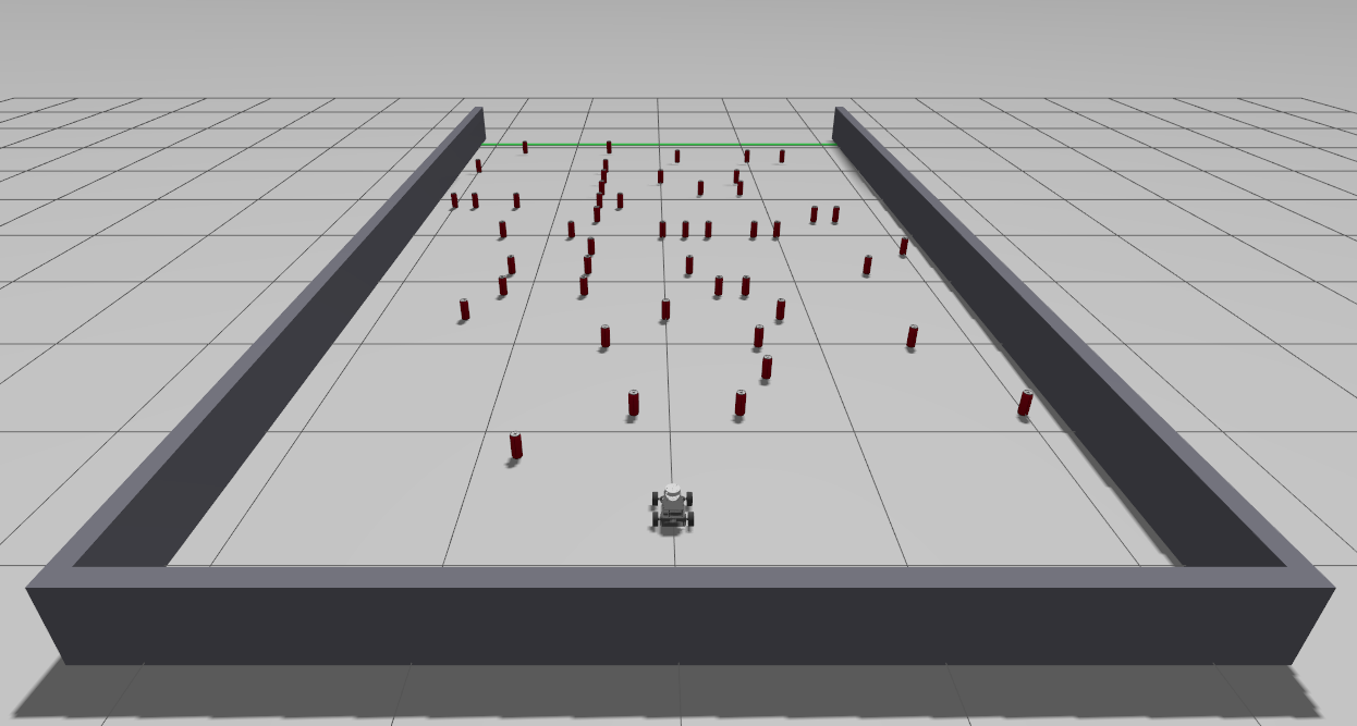
Training on a fixed layout would encourage memorisation, so layouts are randomised per episode. Unrestricted randomness, however, generates unsolvable tasks and contaminates both the demonstrations and the returns. The generator therefore treats solvability as a generation-time acceptance test:
- Sample active cone positions from a fixed pool of 64 locations.
- Mark occupied cells on a planning grid and inflate obstacles by a difficulty-specific clearance radius.
- Run eight-connected A* from start to the goal reference. Diagonal moves are rejected when either adjacent cardinal cell is blocked, which prevents corner cutting.
- Accept the layout only if a route exists that also meets minimum requirements on straight-path blockage and lateral detour.
The validation path is then discarded. It is never observed by the policy, so a solvable layout does not come with a visible empty channel drawn through it.
| Difficulty | Active cones | Centre blockers | Inflated clearance | Lateral detour |
|---|---|---|---|---|
| Easy | 32–40 | at least 1 | 0.28 m | at least 0.30 m |
| Medium | 40–48 | at least 3 | 0.30 m | at least 0.50 m |
| Hard | 48–58 | at least 4 | 0.32 m | at least 0.70 m |
Medium is the default training and evaluation distribution, and every result on this page is reported on medium mazes.
Part II: Imitation
6. Why imitate before reinforcement learning
The first attempt at this task was direct reinforcement learning from a randomly initialised policy. It failed repeatedly, and the reason is structural rather than incidental.
An episode terminates in success only if the vehicle crosses a 7.2-metre obstacle field without contact. A randomly initialised policy essentially never does this. The consequence is not merely that learning is slow: the policy receives no information that distinguishes a trajectory which nearly succeeded from one that failed immediately, because both return the same terminal failure. There is no gradient of improvement to follow. The exploration problem is degenerate, not just difficult.
The response was to write a deterministic expert controller that navigates from the same LiDAR observation available to the learner, and to use it as a starting point. The learner imitates the expert first and is then improved by reinforcement learning.
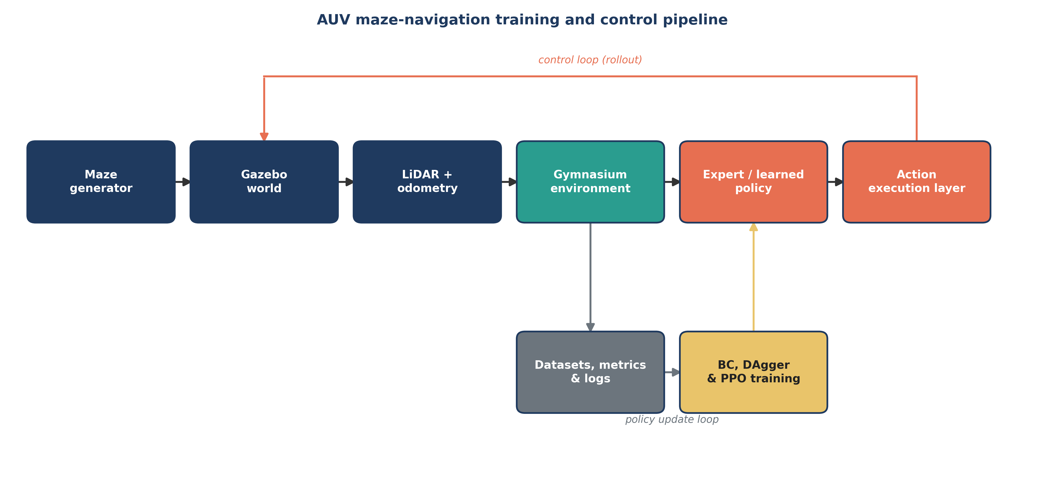
The methodological justification for this ordering is that it eliminates the exploration problem rather than mitigating it. The policy is never asked to discover a successful trajectory; it begins from one and is asked only to refine it. The reinforcement learning stage is thereby reduced from a search over the full policy space to a local improvement of an already competent policy, which is a far more tractable problem — and, as Section 14 shows, one where excessive exploration is a bigger hazard than insufficient exploration.
7. The expert controller
The expert is deliberately simple. It divides the 360-degree scan into four approximately 90-degree sectors — forward, left, right and rear — and moves forward when the front sector has sufficient clearance. Otherwise it selects a lateral direction using the current clearance and the previous avoidance side, and retreats if it must.
| Parameter | Value |
|---|---|
| Sector layout | 4 sectors of ~90° |
| Movement clearance | 0.30 m |
| Minimum forward speed ratio | 0.25 |
| Slowdown range | 0.10 m |
| Control rate | 20 Hz, matching the sensor |
The expert normally translates and does not yaw; it keeps a lateral preference across decisions as hysteresis, so it does not oscillate between two equally good sides.
Its limits shape everything downstream. Around locally ambiguous obstacles the expert can oscillate or time out. That is exactly the failure mode DAgger is designed for, and it is why the pipeline does not stop at behaviour cloning.
The expert returns normalised requested actions, so it uses the same interface as the neural policy. Collection calls the environment’s direct expert step, so demonstrated actuator behaviour matches the comparison node rather than passing through the learner’s smoothing filter.
8. Behaviour cloning
Given expert pairs $(o_i, a_i^E)$, behaviour cloning minimises the squared error between the expert’s action and the mean of the PPO Gaussian actor:
\[L_{BC}(\theta) = \frac{1}{N}\sum_i \lVert \mu_\theta(o_i) - a_i^E \rVert_2^2\]Two details matter more than the loss itself.
The first is that the target is the actor’s mean network rather than a standalone regression head. The result is saved directly in PPO-compatible format, so fine-tuning resumes from a working actor rather than translating between two representations.
The second is the train/validation split, which is performed by episode rather than by transition. Splitting randomly at the transition level would leak neighbouring observations of the same trajectory across the boundary and report a validation error that is optimistic by construction.
| Setting | Value |
|---|---|
| Network | MLP with two hidden layers of 128 units |
| Optimizer | PyTorch Adam |
| Gradient clipping | norm 0.5 |
| Epochs | 50 |
| Train/validation split | by episode |
| Initial action standard deviation | 0.30 |
PPO’s default action standard deviation is broad, which is appropriate when the actor must explore from scratch. Here the actor is already competent, so a broad default would mean destructive exploration at the very start of fine-tuning. Initialising it to 0.30 keeps the policy close to the demonstrations while still permitting improvement.
9. Dataset aggregation (DAgger)
Behaviour cloning alone trains only on states the expert visits. The learned policy will inevitably reach states outside that distribution — the standard covariate shift problem of imitation learning — and its behaviour there is unconstrained by the training objective. A small mistake moves the student somewhere the expert never demonstrated, and there is no training signal covering what to do next.
Dataset aggregation addresses this directly. The student drives; the expert labels each visited state; the policy is retrained on the union of the old and new data. Each round extends the training distribution toward the states the policy actually reaches.
Three rounds were run, raising the student-control probability each time:
| Round | Student-control probability | Safety hand-back |
|---|---|---|
| DAgger 1 | 0.35 | minimum scan ≤ 0.24 m |
| DAgger 2 | 0.70 | minimum scan ≤ 0.24 m |
| DAgger 3 | 1.00 | minimum scan ≤ 0.24 m |
Two collection decisions matter. Failure episodes are retained. This is the opposite of the initial expert collection, and it is the point of the method: collision-adjacent and recovery states are precisely the missing data. Only worker_restart episodes are excluded, because those are infrastructure artefacts whose transitions do not represent policy behaviour at all.
Collection is sharded across four independent workers, each owning its own ROS domain, Gazebo partition, deterministic seed stream and diagnostic log. The parent combines shards only after all workers finish, which avoids pushing large trajectory arrays through multiprocessing pipes.
One question that comes up is whether an expert with four cardinal behaviours caps the learned policy at four actions. It does not. The actor is continuous, the environment filters its commands, and PPO subsequently optimises without the cloning loss. The policy can interpolate between demonstrated actions, and it can discover simultaneous x/y/yaw commands that improve the reward — which is precisely what the diagonal reach described in Section 3 allows.
The full production pipeline used 500 expert episodes, 100 episodes per DAgger round, BC_EPOCHS=50, DAGGER_EPOCHS=15, on medium difficulty with four collection workers at seed 12301.
Part III: Environment Correctness
The largest single improvement obtained during this project came from correcting the simulation environment rather than from any change to the learning algorithm. This part documents the three faults, the evidence that identified each, and what each one implies beyond its own fix.
The reason this deserves its own part is that environment faults present themselves as policy failures. A learner terminated too eagerly, or one that begins an episode acting on the previous episode’s geometry, is externally indistinguishable from a learner that simply cannot solve the task — and no training curve will tell the two apart.
10. The collision threshold
Collision was detected from the closest LiDAR return: an episode terminated if any range measurement fell below a configured threshold, initially 0.20 m.
Under that configuration the expert controller — the same controller, unchanged — scored 20%.
| Metric | 0.20 m threshold | 0.15 m threshold |
|---|---|---|
| Episodes | 20 | 20 |
| Successes | 4 | 17 |
| Collisions | 14 | 0 |
| Timeouts | 2 | 3 |
| Success rate | 20.0% | 85.0% |
| Mean steps | 298.2 | 550.7 |
| Median steps | 200 | 520 |
| Mean minimum scan | 0.199 m | 0.190 m |
| Labelled transitions | 5,965 | 11,014 |
The failing episodes had a mean minimum scan of 0.199 m — immediately at the threshold. The vehicle was not making contact with obstacles. It was being terminated for approaching them. The threshold exceeded the approximate robot width, and a LiDAR range measurement is a distance to the nearest surface along a ray, which is not the same quantity as the vehicle footprint’s clearance to that surface. At oblique incidence the two differ substantially.
Reducing the threshold to 0.15 m raised expert success from 20% to 85% and changed the composition of the residual failures completely: from apparent collisions to genuine timeouts. Mean episode length nearly doubled, because trajectories that previously ended at the collision boundary were now allowed to continue.
The implication extends well past this parameter, and it is the transferable lesson of the section. A policy that is terminated for approaching an obstacle cannot learn to pass close to one. Every narrow gap in every training layout becomes unrepresentable in the learned behaviour, because the states required to traverse it are pruned from the experience before the policy ever sees them. The environment was not merely imprecise — it was actively excluding the behaviour the task requires.
11. Reset synchronisation
The second fault produced records that were, on their face, impossible. Successful episodes were occasionally logged with minimum scans of 0.090 m and 0.117 m under a rule that should have terminated anything at or below 0.15 m. These readings could not be attributed to sensor noise; the records were internally inconsistent.
The cause was a race condition in the reset sequence. The composite termination condition could evaluate a LiDAR scan generated before the vehicle had been repositioned for the new episode. The result was that the first observation of an episode corresponded to the terminal state of the preceding one, and the policy would begin each episode acting on the geometry of the previous layout.
The fix was a two-stage reset that requires fresh sensor data to be received before an episode is considered to have begun. Verification collected 40 exact-expert easy-maze episodes across four workers:
| Metric | Result |
|---|---|
| Attempted / retained episodes | 40 / 40 |
| Successes | 36 |
| Timeouts | 4 |
| Collisions | 0 |
| Success rate | 90.0% |
| Mean minimum scan | 0.196 m |
| Labelled transitions | 20,900 |
No episode contained an implausible minimum scan. All four failures were time limits, and the last surviving category of error was therefore the genuine one — the expert’s own tendency to stall in ambiguous geometry — rather than a simulator artefact.
12. The exact actuation contract
The third fault was the quietest and, in a sense, the most dangerous.
The expert’s commands were passing through the same filter applied to the learner’s commands, and the demonstrations were recording the filtered output rather than the expert’s intended command. The learner was being trained to predict actions the expert had never selected. Wherever the expert asked for a larger command than the filter had so far reached, the recorded label was interpolated toward the previous applied command instead of matching the request.
The magnitude of the discrepancy was modest. Its consequence was not, and the reason is worth stating precisely: nothing in the training signal indicates that the labels are corrupted. The loss decreases, the validation error falls, the policy converges cleanly — to a systematically biased target that it has no way to correct. A defect in the observation or the reward at least leaves a signature somewhere. A defect in the label is invisible from inside the training loop.
The correction was to execute expert commands directly during demonstration collection, so that each recorded action is exactly the action that produced the recorded transition. The environment now retains both the raw requested action and the action actually executed, and logging both is what made the discrepancy visible in the first place.
The general requirement this illustrates is worth more than the specific fix: in imitation learning, the recorded action and the executed action must be identical, and any component interposed between the demonstration source and the actuator must be accounted for — or, better, removed from the path.
Part IV: Results
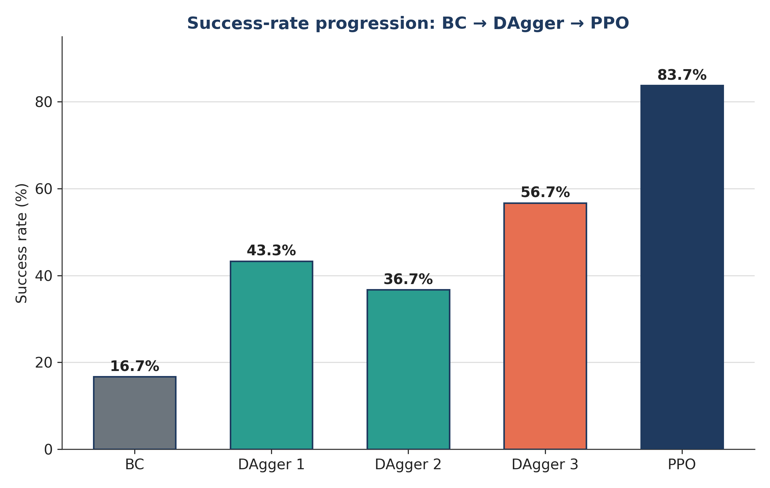
13. Imitation progression
All four imitation checkpoints were evaluated deterministically for 30 episodes on a fixed medium-difficulty block at seed 192301.
| Model | Successes / collisions / timeouts | Success rate | Mean return | Return SD |
|---|---|---|---|---|
| Behaviour cloning | 5 / 25 / 0 | 16.7% | −17.582 | 28.743 |
| DAgger 1 | 13 / 16 / 1 | 43.3% | 5.725 | 36.632 |
| DAgger 2 | 11 / 19 / 0 | 36.7% | 2.057 | 34.040 |
| DAgger 3 | 17 / 13 / 0 | 56.7% | 15.748 | 36.124 |
Behaviour cloning reached 16.7%, which confirms that the demonstrations carry a usable but insufficient signal on their own. DAgger took the same architecture to 56.7% — a gain of 40 points over cloning, and a reduction in collisions from 25 to 13.
The progression is not monotonic: DAgger 2 regressed to 36.7%, below round 1, before round 3 recovered. Round 2 raised student control from 0.35 to 0.70, so more of the collected data came from the student’s own — still imperfect — distribution. The round number is not a proxy for quality, and the rising validation MSE across rounds (0.0144 → 0.0362 on the smoke pipeline) is not a measure of worse control either, because each round adds harder student-visited observations and changes the data distribution underneath the metric. MSE values computed on different aggregate datasets are not a policy ranking.
The practical conclusion is that round number and validation MSE cannot replace held-out navigation evaluation. Only the success rate on a fixed block answered the question that was actually being asked, and it is what selected DAgger 3 as the PPO initialisation.
14. PPO fine-tuning
PPO was selected for the final stage because it handles continuous Box actions, supports vectorised environments, and clips the probability ratio between successive policies — which is exactly the property wanted when refining an actor that is already competent.
| Hyperparameter | Value |
|---|---|
| Network | MLP [128, 128] |
| Rollout length per worker | 512 transitions |
| Workers | 4 |
| Transitions per rollout | 2,048 |
| Batch size | 256 |
| Discount $\gamma$ | 0.99 |
| GAE $\lambda$ | 0.95 |
The clipped surrogate objective limits how far one update can move the policy:
\[L^{clip} = \mathbb{E}\left[\min\left(r_t A_t,\ \operatorname{clip}(r_t,\, 1-\epsilon,\, 1+\epsilon)\,A_t\right)\right], \qquad \epsilon = 0.2\]14.1 A healthy-looking run that did not improve the policy
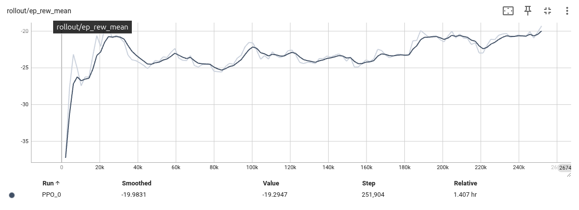
The first full fine-tuning run resumed DAgger 3 at learning rate 1e-4 with four medium-maze environments over a requested 250,000 additional transitions. At its midpoint — 124,928 transitions — its diagnostics read as follows:
| Diagnostic | Observed value | Interpretation |
|---|---|---|
| Throughput | ~50–55 transitions/s | Mechanically stable four-worker simulation |
| Mean rollout reward | ~−24.2; plateau −22 to −25 | Early rise from about −37, then no continued gain |
| Approximate KL | 0.0100 (range 0.005–0.013) | Within a plausible PPO update range |
| Clip fraction | 0.0322 (range 0.03–0.15) | Updates not dominated by clipping |
| Explained variance | 0.575 | Critic fit returns reasonably at times |
| Policy standard deviation | rose from 0.300 to 0.317 | Exploration was growing rather than settling |
| Worker crashes | none | Simulator infrastructure healthy |
Every optimisation statistic is healthy. The loss is stable, successive policies stay close to one another, the value estimates are sensible, and no worker failed. The reading is “training is stable but the policy is plateauing”, not “the policy is healthy”. The rising action standard deviation is the tell: exploration was becoming more aggressive on a policy that was already competent and did not need to explore.
The generalisation: optimisation statistics describe whether learning is proceeding stably, not whether the policy is improving at the task. When the objective is to refine an already good policy, excessive exploration is more hazardous than insufficient exploration, because it displaces the policy from the behaviour that is known to work.
14.2 Teacher-anchored PPO
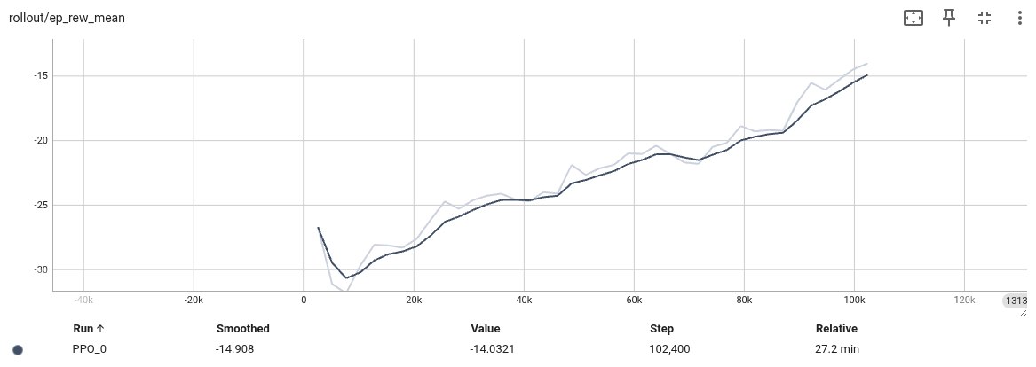
The response was to add a penalty anchoring the actor to its starting point. After each normal PPO update, the actor’s mean-network parameters are interpolated toward a frozen teacher:
\[\theta_{actor} \leftarrow (1 - \beta)\,\theta_{actor} + \beta\,\theta_{teacher}, \qquad \beta = 0.02\]Only mlp_extractor.policy_net and action_net are anchored. The value network and the Gaussian log_std remain free to learn, so the critic can still adapt while the actor stays close to the behaviour that works. The teacher is deliberately not serialised into each checkpoint and must be reattached on continuation.
This is a parameter-space regulariser, not a behaviour-space constraint. It is not a KL trust region and it is not a safety proof: the same parameter displacement can produce different behavioural change in different states. What it does reliably is preserve useful weights while the critic adapts.
| Setting | Value |
|---|---|
| Learning rate | 2.5e-5 |
| Teacher anchor strength $\beta$ | 0.02 |
| Entropy coefficient | 0 |
| Action standard deviation | retained from the checkpoint, about 0.18 |
| PPO clip range | 0.10 |
| PPO epochs per rollout | 5 |
| Target KL | 0.01 |
Note that the entropy bonus is switched off entirely, the learning rate drops by roughly four times, and the clip range tightens from the 0.2 default to 0.10. Every knob is turned toward less change per update. The target-KL value here is an early-stop condition inside a PPO update, not a learning-rate schedule.
14.3 Checkpoints must be selected by measured performance
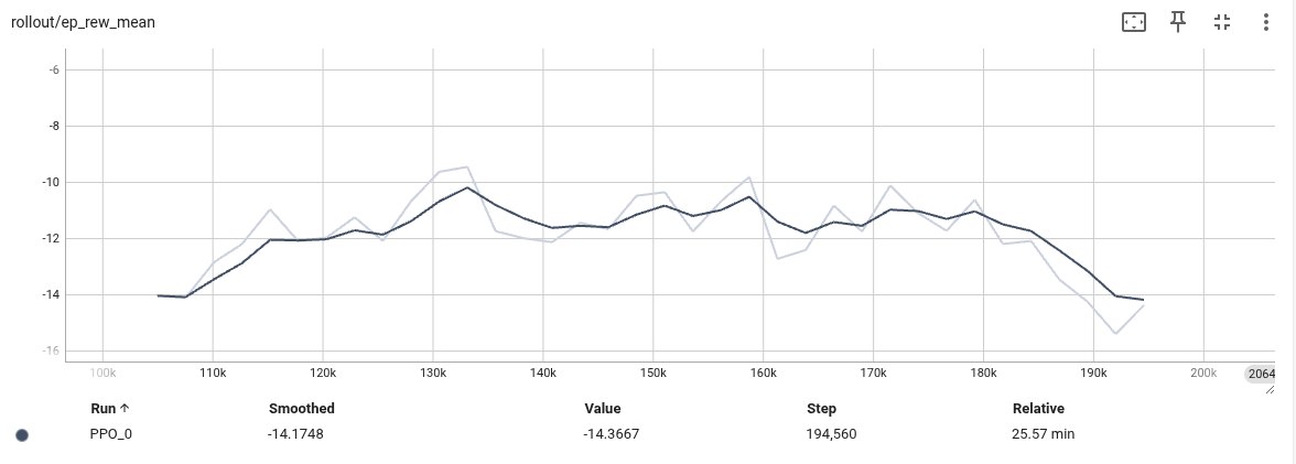
Taking the final or highest-timestep checkpoint as the result is tempting, and one retained anchored run shows the cost: its final_model.zip was evaluated for 100 medium episodes at seed 292301 and scored 45.0% — 45 successes, 53 collisions, 2 timeouts, mean return 6.806, mean episode length 442.42 decisions. That is worse than DAgger 3 on the earlier block and far worse than the champion.
Learning is not monotonic. The champion is therefore the 132,400-step checkpoint of the anchored extension, chosen because it measured best on held-out evaluation — not because it was the last file written or the largest by timestep. The safe workflow this implies is to preserve the teacher and every intermediate checkpoint, and rank them all deterministically.
15. Champion versus DAgger 3
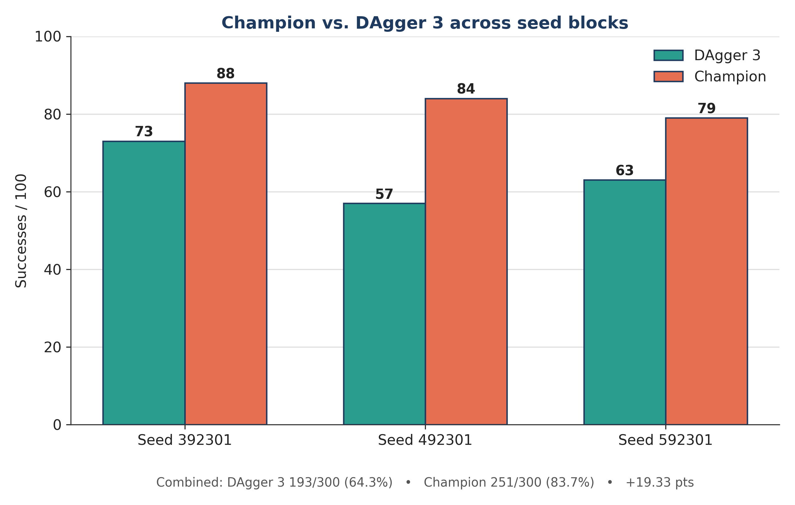
The headline comparison: the champion checkpoint against the DAgger 3 policy it was fine-tuned from, across three 100-episode medium-maze blocks.
| Base seed | DAgger 3 | Champion | Gain |
|---|---|---|---|
| 392301 | 73/100 | 88/100 | +15 points |
| 492301 | 57/100 | 84/100 | +27 points |
| 592301 | 63/100 | 79/100 | +16 points |
| Combined | 193/300 (64.3%) | 251/300 (83.7%) | +19.33 points |
The champion’s pooled 95% interval is [0.791, 0.874].
Across the three blocks DAgger 3 failed 107 episodes and the champion failed 49 — a reduction of 58 failures, or 54.2%. Expressed relative to DAgger 3’s success rate, the champion is about 30.1% higher. The gain is present in all three blocks rather than being carried by one favourable seed range, which is the property that makes it worth reporting at all.
Return statistics move in the same direction, and the spread tightens:
| Base seed | Model | Mean return | Return SD | Mean episode length |
|---|---|---|---|---|
| 392301 | DAgger 3 | 28.527 | 32.046 | 435.26 |
| 392301 | Champion | 38.729 | 24.305 | 453.98 |
| 492301 | DAgger 3 | 15.338 | 37.142 | 398.15 |
| 492301 | Champion | 35.174 | 26.923 | 463.22 |
| 592301 | DAgger 3 | 19.893 | 36.237 | 417.45 |
| 592301 | Champion | 31.886 | 29.637 | 463.53 |
Combined mean returns are 21.253 for DAgger 3 and 35.263 for the champion, with the return standard deviation falling roughly five points. The champion’s longer mean episode length is not evidence of inefficiency: successful routes naturally run longer than episodes that end in an early collision, and the champion solved many more mazes. Any efficiency claim has to be made on mutual successes — episodes both policies solved — using measured simulation time. Those measurements were not collected at this stage.
16. Replication
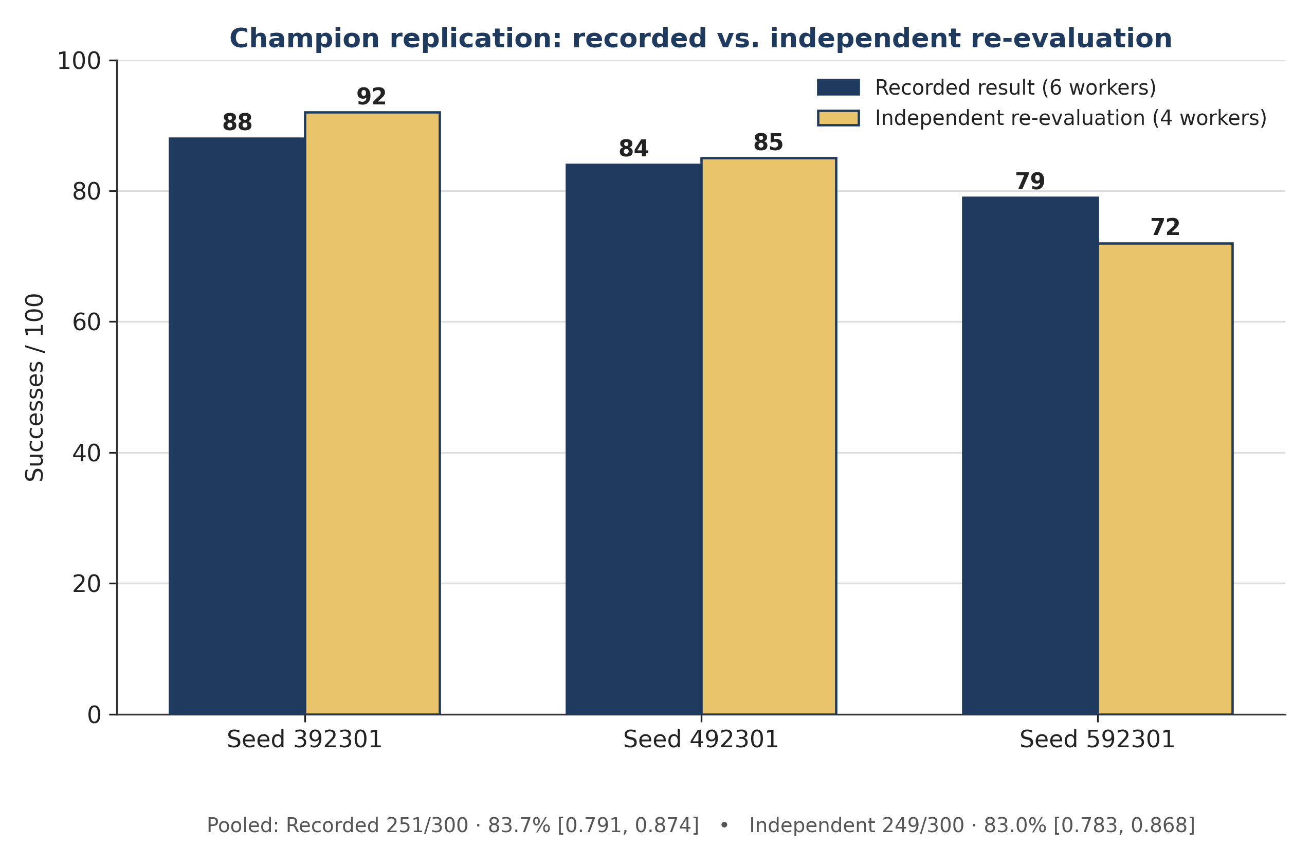
A success rate is only meaningful alongside the protocol that produced it, so the champion’s headline number was re-measured rather than assumed. The same frozen 132,400-step checkpoint was evaluated on the same three seed blocks three separate times:
| Evaluation | Workers | 392301 | 492301 | 592301 | Pooled |
|---|---|---|---|---|---|
| Recorded result | 6 | 88 | 84 | 79 | 251/300 · 83.7% [0.791, 0.874] |
| Independent re-evaluation | 4 | 92 | 85 | 72 | 249/300 · 83.0% [0.783, 0.868] |
The pooled figure moved by 0.7 percent across 300 episodes, against a regression bar of 5 points that had been declared in advance. The two intervals overlap almost entirely.
The per-block movement is not irreproducibility. Block 392301 scored 88 with six workers, 92 with four. Episode seeds are base + episode_index regardless of worker count, so the layout set is identical in all three runs. What changes is which Gazebo process runs which episode and how the asynchronous real-time dynamics interleave. A 6-to-4 worker change alone moves a block by up to 7 points, which is larger than the pooled effect it sits inside. Per-block comparisons should be made at matched worker counts; the pooled figure is the more stable quantity.
Two caveats belong with this result, and neither undermines it.
First, this replicates the evaluation of a frozen model, not the training. PPO training at seed 2301 has never been re-run and re-scored, so the champion’s training remains a single run; what is established is that the champion’s measurement is stable. That is still enough to put the 19.33-point margin over DAgger 3 on firm ground — it is more than four times the ±4.2-point half-width of the pooled interval.
Second, the three blocks used here were inspected during model selection, so they are development and validation data. They are not a pristine final holdout, and describing them as one would overstate the claim.
Part V: Discussion
17. Findings
Three results transfer beyond this task.
The environment is a component of the experiment. The largest single gain in the project — expert success rising from 20% to 85% — came from changing a collision threshold, not from changing the learner. A learner terminated too eagerly, or one that begins an episode on the previous episode’s geometry, is indistinguishable from a learner that cannot solve the task, and training curves will not separate them. The 20%-to-85% probe was cheap and would have been worth running first.
Healthy optimisation statistics do not demonstrate a better deterministic policy. The first PPO run was stable under every diagnostic being monitored while its deterministic performance plateaued. Nothing computed from the learning process reported a defect, because there was no defect in the learning process — the objective and the diagnostics were both working correctly, and neither was measuring the thing that mattered.
A success rate is meaningful only alongside its protocol. Here that means the maze block, the seed, the sampling regime and the worker count. The 0.7-point pooled movement and the exact block reproduction are what license treating 83.7% as an established figure rather than a fortunate draw.
The common thread is that in reinforcement learning the environment, the objective function and the measurement protocol are each part of the model, and each can be wrong in a way that looks exactly like a policy that failed to learn. Finding those faults is slower and less satisfying than tuning the algorithm. In this project it was also the work that produced the difference.
18. Limitations and further work
The principal limitation is that the PPO training run is a single seed. The evaluation of the resulting model has been replicated and is stable, but the training itself has not been repeated and re-scored. A different seed could plausibly produce a materially different checkpoint, and nothing in this work estimates how much.
The second limitation is structural rather than statistical: the policy inherits the expert’s assumptions. Fine-tuning performs local improvement, not global search, so any strategy the expert does not exhibit is effectively out of reach. The expert is reactive and translation-dominant, and it does not yaw — which likely biases the learned policy away from useful rotational manoeuvres in tight geometry, since rotational behaviour has to be discovered by PPO rather than demonstrated.
Third, the three evaluation blocks were used for model selection and are therefore not a pristine holdout.
The most valuable next experiment follows directly: multi-seed replication with a common held-out block, each configuration run several times and the distribution of results reported alongside its central tendency. Only then can a comparison between two configurations distinguish an effect from run-to-run variability. Alongside it, two reporting practices are worth adopting as defaults — naming the evaluation protocol with every figure, and pre-declaring the decision thresholds before the runs rather than after.
Where this left off. A later stage of the project asked whether the same task could be learned without expert supervision at all. Four generations of soft actor-critic training did not produce a working controller up to now.
References
- Schulman, J., Wolski, F., Dhariwal, P., Radford, A., & Klimov, O. (2017). Proximal Policy Optimization Algorithms. arXiv:1707.06347.
- Schulman, J., Moritz, P., Levine, S., Jordan, M., & Abbeel, P. (2016). High-Dimensional Continuous Control Using Generalized Advantage Estimation. ICLR.
- Ross, S., Gordon, G., & Bagnell, D. (2011). A Reduction of Imitation Learning and Structured Prediction to No-Regret Online Learning. AISTATS.
- Raffin, A., Hill, A., Gleave, A., Kanervisto, A., Ernestus, M., & Dormann, N. (2021). Stable-Baselines3: Reliable Reinforcement Learning Implementations. JMLR 22(268).